Chapter 1: Technology Overview

Technology Overview. Airborne Light Detection and Ranging (LiDAR) System, sometimes referred to as Airborne Laser Scanning (ALS), is a remote sensing technique used to measure the distance to an object by determining the time of flight for an emitted laser beam. A scanning mechanism (such as an oscillating mirror) is normally employed to steer a series of laser pulses (typically over 100 KHz) over a wide area from an airborne platform. All airborne LiDAR systems use enabling technologies such as Global Positioning System (GPS) and Inertial Measurement Unit (IMU) to determine the location and orientation of the remote sensor located on the airborne platform (see Figure 1-1). The resulting data are typically used to measure topography of the land surface, including bare earth topography that excludes buildings and vegetation.

1. Operating Principles. Although most commercially-available Airborne LiDAR Systems use a pulsed laser source, there are other operating modes of laser-based remote sensing systems. For example, a laser system can be characterized as a continuous wave (CW) laser system that transmits a continuous signal, and ranging is determined by modulating the intensity of the laser light. In such a system, a sinusoidal signal is received with a time delay. The travel time is directly proportional to the phase difference between the received and transmitted signal. Pulsed laser systems, on the other hand, transmit a series of laser pulses and measure the round-trip time of each laser pulse that scattered back to the optical receiver. The distance (or range) to the target is determined by the one-way time of flight of the laser pulse multiplied by the speed of light.
   1. Laser. The laser ranging unit in airborne laser scanning will include the actual laser; the transmitting and receiving optics; and the receiver with its detector, time counter and digitizing unit.
   2. Laser Wavelength. For topographic mapping using airborne laser scanning, where high energy pulses are required to perform distance measurements over long ranges, only certain types of solid-state, semiconductor, and fiber lasers have the specific characteristics – ability to produce high intensity collimated beams – that are necessary to carry out these operations. Nearly all airborne topographic LiDAR systems that use solid-state crystalline material such a neodymium- doped yttrium aluminum garnet (Nd:YAG) lasers operate in the near-infrared wavelength range (typically 1064 nm). Fiber lasers (sometimes referred to as glass lasers) operating at or near 1550 nm have also been routinely used, though these systems operate at lower power levels and cannot reach the same operating altitudes as the 1064 nm laser sensors. Lasers have also been developed to operate at 905 nm, but are not very popular for airborne LiDAR applications due to their low- intensity returns over saturated sediments. Another class of lasers operates at the frequency- doubled blue-green wavelength of 532 nm. These sensors are typically used in bathymetric and topobathymetric applications because the green-wavelength laser is able to penetrate through the water column under certain conditions; see Chapter 7 for more details.
   3. Pulse Energy, Pulse Width, and Beam Divergence. The pulse energy, measured in micro Joules (µJ), is simply the total energy of the laser pulse. Pulse duration, measured in nanoseconds (ns), is typically defined as the time during which the laser output pulse power remains continuously above half its maximum value. Beam divergence, measured in milliradians (mrad), refers to the increase in beam diameter that occurs as the distance between the laser instrument and a plane that intersects the beam axis increases. The pulse energy of topographic LiDAR systems are typically low (10-100 µJ) to allow for a tightly focused beam with low beam divergence that is also eye safe. Bathymetric LiDAR systems have pulse energies up to 7 mJ, which are typically much higher than the near-infrared lasers used in topographic applications. The higher power is needed for the laser pulse to penetrate through the water column to map the bottom. The bathymetric sensors with very high laser pulse power also have a large footprint so that the energy is spread across a larger area for eye-safety reasons. The pulse width determines the range resolution of the pulse in multiple return systems (explained below), or the minimum distance between consecutive returns from a pulse. Traditionally, pulse widths for topographic systems have been in range of about 10 ns. This means that there is a “blind spot” of about 1 meter along the laser path behind each received LiDAR return. Newer laser technology has enabled the use of much shorter pulse widths (1-2 ns) for topographic and topobathymetric applications. For topobathymetric applications, a short pulse width laser enables the separation of a return from the water surface and bottom in very shallow water depths. This limits the effective measurement depth to >0.5m for threshold detect topobathy LiDAR systems.
   4. Pulse Repetition Frequency (PRF). The PRF, measured in kHz, is the number of pulses emitted by the laser instrument in 1 second. Older instruments emitted a few thousand pulses per second. Modern systems can support frequencies of 400 kHz and newer technologies are now enabling 2 lasers channels to be used in conjunction with the same scanning mirror, thereby producing effective PRF of 800 kHz. Many systems allow different settings for the PRF. This is usually done to allow the systems to fly at different flight altitudes.  The PRF is directly related to the point density on the target. For example, a system operating at 167 kHz from the same flying altitude will have higher number of returns than when operating at 100 kHz. Equivalently, a high PRF system can generate desired return densities by operating on an aircraft that flies higher and faster than an aircraft carrying a lower PRF system, thereby reducing flying time and acquisition costs when weather conditions allow for higher flying altitudes.
2. Scanner. The primary goal of the scanning technique is to create a wide swath with consistent along- and across-track point spacing, and reliable and accurate elevations for the entire swath. Several scanning techniques have been used in airborne LiDAR systems. In theory there are no special reasons why one scanning technique is preferable to another, although scan patterns that facilitate constant incident angle on the terrain can reduce data voids related to dynamic range of the receiving optics. The most common scanning techniques are the Oscillating Mirror and Rotating Mirror.
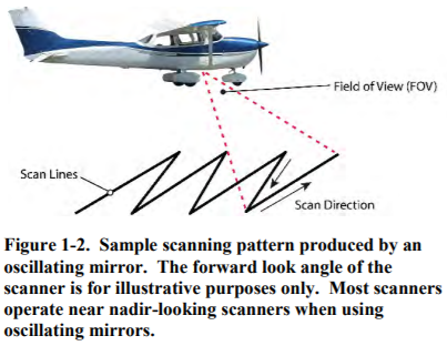   1. Oscillating Mirrors. In systems using an oscillating mirror, the mirror rotates back and forth between limited extents, producing a zigzag (i.e. sinusoidal pattern) line on the surface of the target area (Figure 1-2).  The mirror is always pointing downwards towards the ground so data collection can be continuous and theoretically all pulses of the laser can be used. The field of view and scan rate can be set by the operator prior to acquisition. Changing the field of view provides additional flexibility as it allows laser pulses to be collected over a shorter span (denser data ) or a wider span (sparser data). Although the oscillating mirror is the most widely used scanning mechanism for airborne LiDAR systems, there are inherent disadvantages of using the oscillating mirror principle. The changing velocity and acceleration of the mirror as it oscillates from one end to the other causes unequal spacing of the laser pulses on the target. The point 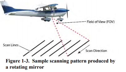density increases along the edges of the scan where the mirror slows down, and decreases along the center in the along-scan direction. The forward motion of the aircraft causes the zig-zag pattern with varying point spacing along the edges of the scan in the cross-scan direction. Manufacturers have solved these problems by essentially ignoring the outlier points on a scan and modeling the distortions caused by changing speed using a computer algorithm.
   2. Rotating Mirrors. The rotating mirror is another commonly used scanning mechanism for airborne LiDAR systems. In this approach, the mirror is rotated continuously at a constant velocity in one direction producing
   3. a parallel line scan (Figure 1-3). The constant velocity ensures that there are no acceleration type errors encountered in the oscillating mirror scanner. The point spacing is also more regular both along and across the scan. However, the biggest disadvantage is that observations cannot be taken during a significant time during each mirror rotation when the mirror is pointing away from the target. Typically, 30-40% of the emitted laser pulses are not aimed at the target area and are essentially lost to the scanning mechanism.
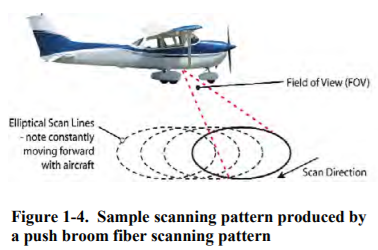
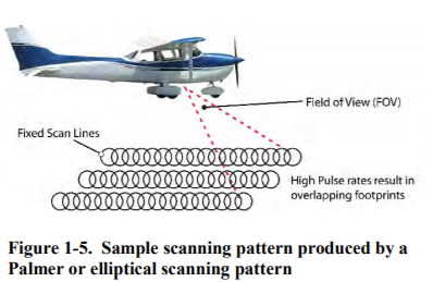
   4. Other Scanning Patterns. Other scanning mechanisms less commonly used include the push broom (fiber scanning) pattern where the laser pulsed energy is transmitted into one of the fibers arranged in a circle producing a nutating scan pattern (Figure 1-4) and the Palmer scanner that produces an elliptical scanning pattern with redundant data that can be used for calibration or to get a forward and aft view of the same target (Figure 1-5).
3. Geopositioning. Calibrating LiDAR data begins with the proper installation/mounting of the LiDAR unit, GPS antenna, and IMU sensor on the aircraft, and the precise measurement of offsets in the x, y, and z directions between each of these sensors. The IMU usually serves as the point of reference and the precise distance between all units are measured with respect to the IMU. The precise location of the GPS base station, the antenna height, and the phase center information are required to process the differential GPS-IMU trajectory. The GPS-IMU trajectory is the precise aircraft trajectory that contains the 6 positioning and orientation parameters: x, y, z, pitch, roll, heading; along with a unique timestamp.  The position  information is derived from post-processing the aircraft GPS receiver data along with the GPS base station data using specialized differential GPS (DGPS) software. The LiDAR positions are calculated at 0.5 second steps. In a second step, an integrated position and orientation solution is calculated with the DGPS-position data and the IMU data by another software module, yielding position and orientation (roll, pitch, yaw) angles to better than one-hundredth of a degree. The IMU measurement rate is typically 200 Hz; the trajectory values are usually maintained at the same rate as the IMU, i.e. 200 records per second. Once the GPS and IMU data are processed and passes all QC checks, the data are combined with the laser range data. This processing step is performed in the LiDAR manufacturer’s developed software. Calibration is done at this stage of the processing. Although the methods of performing calibration are software-dependent (and hence manufacturer-dependent), the LiDAR vendor should test the calibrated data independently. This is usually done by interrogating data from four overlapping flight lines flown in opposite and perpendicular directions along building rooftops and flat surfaces such as airport runways.
   Any misalignment between the IMU and the LiDAR scanner can be determined using this approach. This information can be fed back into the calibration software to improve the overall calibration of the data. Calibration testing is recommended prior to each mission and is necessary when any of the LiDAR system components are remounted on the aircraft. Several different types of airborne LiDAR systems were developed in the research and scientific field since the late 1970s through the 1980s. These systems typically involved the use of laser profilers to generate a single line profile of the ground beneath an aircraft. The development of Global Positioning System (GPS) and Inertial Measurement Unit (IMU) technologies in the 1990s for civilian applications eventually led to the use of airborne LiDAR systems for accurate topographic mapping. The development of laser scanners (explained in Section 1-1.b above) during the same decade also enabled the use of these systems for wide-area topographic mapping. Airborne LiDAR systems can be broadly classified based on the following specifications: (1) Laser wavelength (2) Pulse energy, pulse width, and beam divergence; (3) Pulse Repetition Frequency (PRF); (4) Operating Altitude; and (5) Return type.
4. Operational Considerations
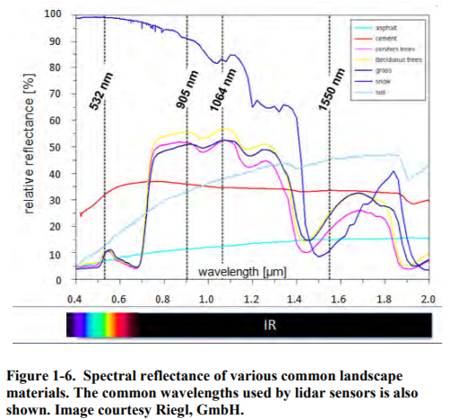   1. Reflectance. Reflectance is an important property that affects LiDAR performance. The amount of energy that arrives back at the LIDAR receiver is directly proportional to the percentage of energy that reflects off the object, or in other words the object’s reflectance. The reflectance of the object is wavelength-dependent, and because LiDAR systems are monochromatic, the reflectance at that particular wavelength determines how detectable an object is given the laser power. Figure 1-6 shows the relative spectral reflectance of various common landscape materials.
   2. Operating Altitude. The operating altitude for an airborne LiDAR system is largely dependent on the required point density of data and the ability of the laser to reliably detect returned energy and determine the elevation of a target at varying reflectivities. Some LiDAR systems are specifically designed as low-altitude sensors with relatively low pulse energy. These systems have typically high PRFs that enable the acquisition of 20-50 points per square meter at operating altitude of 500-3000 ft. Other systems are designed to be used at much higher operating altitudes (3000-8000 ft). These systems are designed for wide-area mapping with swath widths that can extend to 1500 meters. Until early 2006, high-altitude sensors were limited by the inability to track multiple pulses in air (MPiA). For these sensors without MPiA capability, an emitted laser pulse had to bounce off the target and be received by the sensor before the next pulse could be emitted. As a result, the PRF and operating altitude had to be limited in order to have only 1 pulse in the air at any instant of time. Recent developments in firmware now allow the tracking of MPiA, also known as Multiple Time Around (MTA), and some sensors can track up to 8 pulses in the air.  MPiA technology has enabled LiDAR sensors to use 2 laser sources simultaneously (dual-channel lasers), thereby producing 800 KHz PRF and the ability to operate at altitudes of over 7000 ft.
   3. Return Type. Early versions of airborne LiDAR systems were capable of recording only one pulse at low pulse repetition rates. However, more advanced LiDAR systems can record simultaneously multiple returns for each transmitted pulse, and the reflected intensity for each return. Multiple return LiDAR systems are very useful in forestry applications or even to derive bare Earth topography under vegetation. When the laser beam from a multi-return system interacts with a tree canopy, then the first return is usually assumed to arrive from the top of the tree (or where the transmitted laser beam first interacts with the tree canopy). The last return may interact with the ground underneath the tree, although the ability to map the ground is largely dependent on the density of the vegetated canopy. Intermediate returns, perhaps 2^nd, 3^rd, and 4^th, are expected to be caused by tree branches and understory vegetation between the top of the canopy and the ground.

Chapter 2: Project Specifications

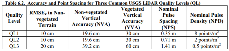
Project Specifications. Numerous sensor parameters affect the desired quality and specifications of the LiDAR data. The USGS LiDAR Base Specification Version 1.2, at Appendix F, provides three of the most common LiDAR Quality Level (QL) specifications relevant to industry QL1 LiDAR (with 1-foot contour accuracy and 8 points/m²), and QL2 LiDAR (also with 1-foot contour accuracy but with 2 points/m²) both ensure that the point cloud and derived data products are suitable for the inter-Agency National 3D Elevation Program (3DEP); whereas QL3 LiDAR (with 2-foot contour accuracy and 0.5 point/m²) ensures that the bare-earth DEMs derived from LiDAR data are suitable for ingestion into the National Elevation Dataset (NED). Using the USGS Lidar Base Specification at any of these three Quality Levels will ensure that it is consistent with the goals of the National Digital Elevation Program (NDEP). Also see the ASPRS Positional Accuracy Standards for Digital Geospatial Data, at Appendix D, from which the Elevation Data Vertical Accuracy Standards were extracted in Chapter 3, Table 3-6. LiDAR point density and vertical accuracy are the two main cost drivers of an airborne LiDAR survey. LiDAR data can be collected with a wide variety of point densities depending on the needs of the project. The selection of point density is a big driver of the overall cost of a LiDAR project and should be selected with consideration to the end uses for the LiDAR. A LiDAR product with 1 point per square meter (ppsm) is sufficient for many applications such as flood mapping in many areas. Higher point densities (4-8 ppsm) allow for greater utilization of the data for mapping planimetric features such as roads and structures as well as for vegetation analysis such as biomass and canopy studies. Additionally, specialized LiDAR at very high densities > 20 ppsm are often used for mapping infrastructure in greater detail such as power lines, pipelines, and for significant features such as mile posts and signs.

The ground conditions should be considered when selecting a point density as well. If the area is covered with dense vegetations such as a coniferous forest a higher density and more overlap would be required to penetrate to the ground than an area where leaf-off conditions exist.

1. Geographic area to be mapped (normally based on government-provided shapefiles);
2. Returns per pulse (typically is 3 or more including, first, last, and intermediate returns);
3. Collection conditions (e.g., ground is snow free, vegetation is leaf-off);
4. Ground control and/or direct georeferencing requirements (airborne GPS and IMU positioning and orientation), if any;
5. GPS base station limitations, if any;
6. Data void guidance, if any (void areas are allowed over open water and typically wet or very new asphalt);
7. Vertical accuracy (using current ASPRS and NDEP methods where NVA is tested as Accuracy_z (RMSE_z x 1.9600) and VVA is tested using the 95^th percentile); NVA and VVA definitions are provided in Chapter 3 of this manual;
8. Horizontal accuracy (normally compiled to meet a specified value rather than tested to meet a specified accuracy value);
9. Relative accuracy (threshold, typically stated in terms of RMSE, of vertical offset between adjacent flight lines);
10. GPS-IMU trajectory solutions should be delivered and assessed for combined vertical separation between the forward and reverse trajectory solutions;
11. Tiling schema including size of final tiles and naming convention (e.g., 1,000 meter grid with no over-edge named according to the U.S. National Grid);
12. Horizontal datum (e.g., North American Datum of 1983 (NAD83)/2011 adjustment);
13. Vertical datum (e.g., North American Vertical Datum of 1988 (NAVD88), using the most recent National Geodetic Survey (NGS)-approved GEOID model for conversions from ellipsoid heights to orthometric heights, currently GEOID12A;
14. Coordinate system (e.g., UTM or State Plane Coordinate System);
15. Vertical and horizontal units (e.g., meters, or U.S. Survey Feet) – note, never specify “feet” but instead specify U.S. Survey Feet or International Feet;
16. What classes are required (e.g. 1-unclassified, 2-ground, 7-noise, 8-model key points, 9- water, 12-overlap, etc) (See section 1-4.c. for a description of classifications);
17. Processing requirements (e.g., percentage of elevated features allowed to remain in the ground classification, guidelines for over-smoothing/inconsistent editing, thresholds for artifacts/spikes/divots/cornrows, uniformity of point distribution);
18. File format (industry standard is LAS format following ASPRS formatting guidelines and specifications);
19. Compression (e.g., are compressed files allowed, if they are to be delivered in addition to or in replacement of non-compressed files, and what format should be used for the compressed files);
20. Ff intensity imagery is required, specify the resolution or pixel size;
21. If breaklines are to be collected, specify types of breaklines, minimum size for collection, monotonicity/connectivity requirements or topology rules that must be followed, and desired final format of the breaklines (e.g. ESRI shapefile, ESRI geodatabase, DXF, DGN, );
22. If DEMs (such as bare-earth DEMs or first return DSMs) are to be created, specify the pixel resolution, hydro-flattening or hydro-enforcement requirements, and final format (ESRI Grid, IMG, GeoTIFF, );
23. If contours are to be created, specify the interval, coding (intermediate, index, etc), level of smoothing to be applied (e.g. engineering grade, moderately smooth, cartographic grade), and the desired final format (e.g. ESRI shapefile, ESRI geodatabase, tiled, non-tiled);
24. Metadata requirements such as those defined in the IAW geospatial manual;
25. QA/QC procedures;
26. Reports to be submitted (e.g., survey report with field work procedures, data acquisition report, calibration procedures, production report, QA/QC report); and
27. Deliverables and due dates.

Please note, however, that industry managers should make every effort to utilize existing ASPRS standards and specifications listed above to ensure that the data will be interoperable, usable and available to others.

Chapter 3: Project Planning

Project Planning. There are numerous requirements to assess when planning a LiDAR project as shown in the specifications section of this chapter. However, regardless of the specific requirements project planning always starts with the basic questions: Why is this dataset needed? What are the specific deliverables that are needed? When are the deliverables needed?

1. Review of Project Specifications. Planning is performed after careful review of the project specifications and answering a series of questions: Should maps be compiled to NAD83 (HARN) for the horizontal datum and NAVD88 for the vertical datum? Should elevation data (orthometric heights) be produced by converting from ellipsoid heights using the GEOID12A model? Should the coordinate reference system use the relevant State Plane Coordinate System or Universal Transverse Mercator (UTM) coordinates? (Note: State Plane coordinates are more accurate for typical requirements). Should the units be feet or meters? If feet, should U.S. Survey Feet or International Feet be used? What should be the nominal point density? What classifications should be included i.e., ground, water, buildings, vegetation, etc? Are planimetric features such as roads or buildings needed to be extracted from the LiDAR data? Are there limits on environmental factors such as shadows, clouds, topography, climate, snow cover, standing water, tidal and river levels? Will DEMs, DSM, Contours, or other derivative products be produced? What are the metadata requirements? How are accuracies to be reported in the metadata; will the accuracy be reported using the accuracy at the 95% confidence level for the NVA? Are waveform data needed? If yes, what is the data format?
   1. LiDAR Point Density. LiDAR data can be collected with a wide variety of point densities depending on the needs of the project. The selection of point density is a big driver of the overall cost of a LiDAR project and should be selected with consideration to the end uses for the LiDAR. Modern LiDAR sensors are capable of acquiring LiDAR data with a higher density than previously available and can do so at higher altitudes and with less overlap. A LiDAR product with 1 point per square meter (ppsm) is sufficient for many applications such as flood mapping in many areas. Higher point densities (4-8 ppsm) allow for greater utilization of the data for mapping planimetric features such as roads and structures as well as for vegetation analysis such as biomass and canopy studies. Additionally, specialized LiDAR at very high densities > 20 ppsm are often used for mapping infrastructure in greater detail such as power lines, pipelines, and for Department of Transportation (DOT) significant features such as mile posts and signs. The ground conditions should be considered when selecting a point density as well. If the area is covered with dense vegetations such as a coniferous forest a higher density and more overlap would be required to penetrate to the ground than an area where leaf-off conditions exist.
   2. Swath Overlap. Planning for swath overlap should also be included in the overall planning of the point density. A higher percentage of overlap may be beneficial in an area with dense vegetation as there will be more look angles from the sensor to the ground at any given points. The result would mean that there could be a lower point density requirement in an individual swath with the overlap accounting for an overall higher point density on the project. Depending on the scanning pattern, data from the extreme edges of the swath may be unusable due to geometric nature of the scan pattern. Typically, 10% overlap between swaths is the minimum requirement for an airborne LIDAR collect. However, most LiDAR flights are conducted with 30% overlap, and those that require higher pulse density in vegetated areas are often flown with 55% overlap.
2. Flight Planning. Flight planning is always the responsibility of the acquisition contractor. Flight planning for LiDAR will vary greatly depending on the sensor utilized for the acquisition. Parameters such as flying height, ground speed, scan rate, scan angle, etc will be different for each sensor. The contractor’s flight plan should be evaluated to ensure there is sufficient swath overlap given the sensor’s scanning mechanism and project accuracy specifications. Typically, 10% overlap between swaths is the minimum requirement for an airborne LIDAR collect. However, most LiDAR flights are conducted with 30% overlap, and those that require higher pulse density in vegetated areas are often flown with 55% overlap. A higher percentage of overlap may be beneficial in an area with dense vegetation as there will be more look angles from the sensor to the ground at any given points. The result would be a lower point density requirement in an individual swath with the overlap accounting for an overall higher point density on the project. Depending on the scanning pattern, data from the extreme edges of the swath may be unusable due to geometric nature of the scan pattern. Table 1-1 below shows the operational parameters for a sample LiDAR project for an Optech ALTM 3100 system. The LiDAR flight planning process is mostly automated after entering basic information such as point density, overlap requirements, and scan angles. Trajectories are planned for each flight line. Furthermore, modern Flight Management Systems (FMS) enable the pilot to fly these trajectories with close tolerance. LiDAR sensors are actively acquiring data throughout the entire flight which requires the aircraft to be consistently ‘on-line’ to ensure full coverage.
   Additionally, sensor operators are often able to view the acquisition in real time and assess areas where voids or sensor anomalies may be present during the flight. While LiDAR sensors also have some forms of stabilization, the roll, pitch and yaw of the aircraft still depends upon wind conditions. Regardless of sensor to be used, flight planning also includes the assessment of military and other controlled air space where special permits may be required. Aviation Sectional Charts are often used to determine flight restrictions and controlled airspace when planning flight lines.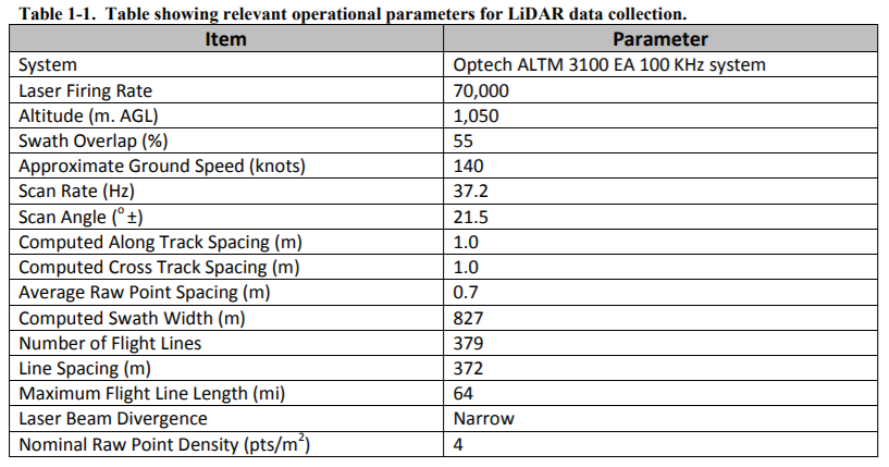
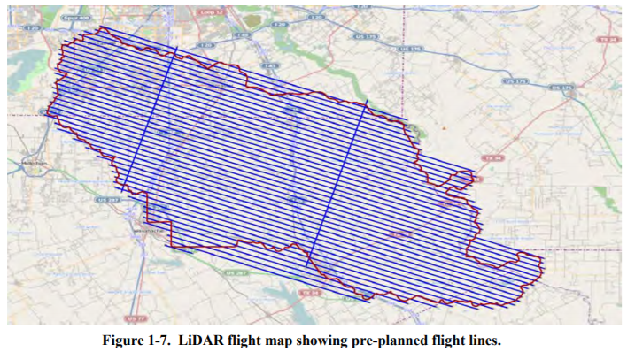3. Acquisition Planning. With LiDAR sensors it is not necessary to specify standard flying heights as the different sensors each have variable requirements for flying height in order to meet project specifications. The principal flight planning parameters then are the point density and overlap required for the project. With LiDAR sensors, storage is handled via ruggedized mass storage usually in the form of removable hard disk drives or flash drives depending on the sensor in use. Figure 1-7 shows a flight diagram with planned flight lines and cross flight lines that are used for calibration.
4. Aircraft considerations. Twin engine aircraft are used most often for airborne LiDAR remote sensing. Twin engine aircraft provide efficient operations for sensors up to 20,000 feet above sea level; they are equipped with power sources to handle a suite of modern sensors; they offer workspace and comfort to the pilot and camera operator; and the twin engines provide additional safety in the event a single engine should stall. Maintenance, operation, ferry and collection costs can be quite variable among different twin engine aircraft. For altitudes above 20,000 feet, performance (cost) is improved when using turboprop or jet aircraft instead of piston aircraft.
5. Survey Control. Three forms of mapping control support airborne LiDAR mapping: airborne GPS control, ground control, and quality control checkpoints. Contract specifications should reference the following standards and guidelines: FGDC-STD-007.4-2002, Geospatial Positioning Accuracy Standards PART 4: Standards for Architecture, Engineering, Construction (A/E/C) and Facility Management, as well as CHAPTER 3 of this manual, Applications and Accuracy Standards, specifically Table 3-6, Elevation Data Vertical Accuracy Standards. Other references relevant to mapping control include EM 1110-1-1002, Survey Markers and Monumentation; EM 1110-1-1003, Navstar Global Positioning System Surveying; and NOAA Technical Memorandum NOS NGS-58, Guidelines for Establishing GPS-Derived Ellipsoid Heights (Standards: 2 cm and 5 cm), version 4.3.
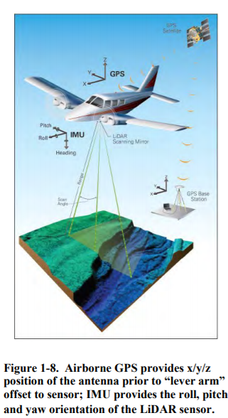
   1. Airborne GPS Control. Airborne LiDAR is acquired with the use of ABGPS for recording the 3D (X/Y/Z) coordinates of each pulse, plus an inertial measurement unit (IMU) for recording the roll, pitch and yaw of the sensor, when each pulse is transmitted and received (see Figure 1-8). When six exterior orientation parameters of each pulse (X/Y/Z and roll/pitch/yaw) are known, requirements for surveyed ground control are greatly reduced. ABGPS receivers must be capable of tracking both coarse acquisition (C/A) and pseudorange (P-code) data. They must provide dual frequency (L1 and L2) and multi-channel capability with on-the-fly ambiguity resolution and be able to log GPS data at 1-second epochs or better. GLONASS receivers capable of receiving satellite information from GPS and GLONASS constellation are preferred over GPS-only receivers.

   

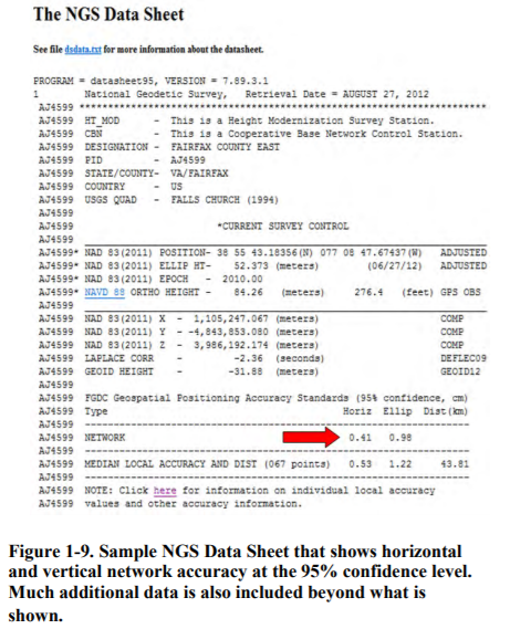
   1. Ground Control. These are the well-established points that GPS ground base stations will be placed on to facilitate accurate positioning of the aircraft In the U.S., this typically involves the use of a Continuously Operating Reference Station (CORS) or the identification and recovery of well-documented permanent control monuments or benchmarks from the National Geodetic Survey’s National Spatial Reference System (NSRS) – (go to http://www.ngs.noaa.gov, then click on Survey Mark Datasheets and/or CORS). If a control network of horizontal control monuments and/or vertical control benchmarks does not exist, a control network will first need to be established per references cited above. Figure 1-9 shows an example NGS Data Sheet with the red arrow point at the horizontal and vertical network accuracy at the 95% confidence level. In addition to data shown here, Data Sheets typically also include additional information such as: State Plane and UTM coordinates; U.S. National Grid spatial address; explanations of how horizontal coordinates, ellipsoid heights and orthometric heights were determined; station description and instructions for finding the monument; station recovery history, etc.
   2. Quality Control Check Points. The quality control checkpoints are typically collected by a survey team independent of the LiDAR vendor so that these checkpoints remain “blind” during the LiDAR acquisition and calibration processing. This can be another contracted party or district personnel. The ASPRS Positional Accuracy Standards for Digital Geospatial Data, at Appendix C, provides detailed guidelines on the number and location of check points. Google Earth or other open source imagery can be used for point selection unless alternative orthophotography is available.
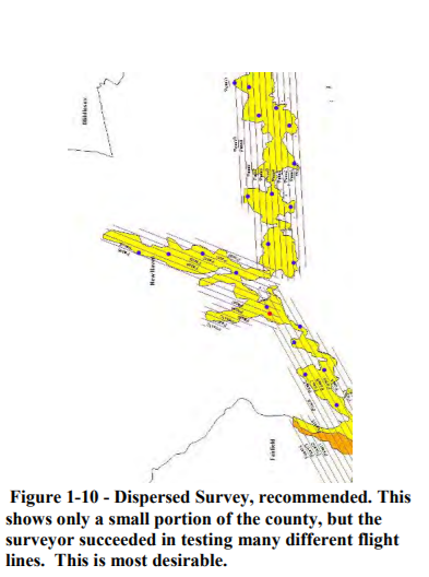
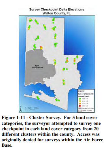
   3. Check Point Distribution. When possible, dispersed surveys (Figure 1-10), which provide a more legitimate assessment of data accuracy throughout the project area for different flight lines, are recommended. For dispersed surveys, no two survey checkpoints should be closer than 5,000 feet from the next closest point. If cost and accessibility are an issue, then cluster surveys can be performed (Figure 1-11). Cluster surveys are typically five points when five land cover categories are being tested, one per category, with a minimum spacing of about 1000 feet between points. Clusters should be dispersed following the ASPRS guideline that at least 20% of the points must be in each quadrant. These types of surveys work best with real-time kinematic (RTK) surveys where a base station can be established and five points (all at least 1000 feet apart from each other) can be surveyed. RTK is also ideal for establishing inter-visible pairs for conventional surveys to establish forest points. Please note inter-visible pairs cannot “count” as check points as they typically do not conform to the minimum distance rule. Furthermore, no two checkpoints in a single cluster should be for the same land cover class, and it is often difficult to identify all five land cover classes within the area of a single cluster.
      
   4. Check Point Location. In addition to land cover classes, location and distribution, the surveyor also needs to avoid known pitfalls in selection of checkpoint locations. It is important for the surveyor to understand that the horizontal coordinates of QA/QC checkpoints do not normally match the horizontal coordinates of individual LiDAR pulses. Instead, LiDAR elevations are interpolated from surrounding points to determine the most probable elevation of the LiDAR data at the horizontal coordinates of each QA/QC checkpoint. Interpolation assumptions are reasonably valid only when the following guidelines are followed with checkpoint selection:
      1. Each checkpoint should be on terrain that is flat or uniformly sloping within 5 meters in all directions from the checkpoint coordinates. Interpolation procedures can fail if the terrain undulates up and down surrounding the checkpoint, or if the slope is curved (concave or convex). Steep slopes should also be avoided for location of checkpoints.
      2. There should be no breakline within 5 meters of a checkpoint. Breaklines define the edge between two intersecting surfaces with different slopes. This rule can best be explained by using a breakline on a bridge abutment as an example of where checkpoints should not be located. Interpolation of LiDAR elevations around a bridge abutment would normally include a point on top of the bridge deck and another point over the side of the bridge, perhaps near water level 10 feet lower; interpolating between these two elevations (even if both LiDAR elevations were perfect) would erroneously show that the LiDAR data had an elevation error of 5 feet.
      3. Similarly, checkpoints, even on flat terrain, should avoid logs, tree stumps, rock piles, or other elevated features that could be mapped by LiDAR pulses within 5 meter of a QA/QC checkpoint.
      4. For survey of checkpoints to be used for horizontal accuracy assessments, surveyors should avoid selecting checkpoints with a high probability of being obscured when mapped with LiDAR (or imagery). Because clearly defined point features are required, horizontal checkpoints are commonly surveyed on corners of paint stripes on asphalt. Such points should not be located under trees (in parking lots) for example, because the black/white intensity variations will not be visible. Similarly, such points should not be selected in actual parking spaces where vehicles are liable to be parked at the time the LiDAR data are acquired.
      5. For these reasons, in spite of check point pre-selection, final checkpoint locations cannot be determined in the office but must be left up to the field surveyor. Flexibility must be given to the surveyor as field conditions, including accessibility, are unknown. The surveyor must use the guidance above to plan where checkpoints are likely to be located, but then must make the final decisions in the field, ensuring points are well spaced, have the correct number of land cover categories, and avoid the pitfalls identified above.

Chapter 4: LiDAR Data Processing

LiDAR Data Processing and Deliverable Development. The range data from the LiDAR sensor are integrated with the aircraft georeferencing (GPS) and orientation (IMU) data to produce a processed laser file, yielding the 3D position and intensity for each laser return. The following sections outline the general steps that are used to process the LiDAR data into some common final deliverables.

1. Data Formatting. After LiDAR acquisition and calibration, LiDAR data are typically processed in order to deliver bare earth classified, LAS files in version 1.2 (formatted to Point Record Format 1) adhering to a specific tiling schema (e.g. US National Tiling Grid) at a specified interval (usually 1,000 m x 1,000 m). Tiles which are fully within the project boundary contain data to the full extent of each tile. Tiles which lie on the project boundary are not filled to the full extent of the tile, unless specified in the scope of work. No over edge data are required but gaps in the data at the project boundary are considered unacceptable. Each LiDAR LAS file (per tile) produced should contain the following elements, as a minimum, for each return:
   1. The return number for each signal
   2. Horizontal and Vertical Position (x,y,z) in the specified horizontal and vertical datum
   3. Intensity return values for each return signal
   4. GPS Timestamp of capture for each point (the timestamp should be unique for each laser pulse)
   5. Georeference information included in the LAS header
2. LiDAR Data Classification. Classification is the process whereby the acquired LiDAR points are filtered, and those representing ground and above ground features (such as trees and buildings) are assigned to separate classes. LiDAR data can be classified into various categories including ground, vegetation, water body, and buildings. Typically, each LAS file is classified as bare-ground or not bare-ground according to the American Society for Photogrammetry and Remote Sensing (ASPRS) LAS format classification table (at a minimum):
   1.  Class 1 – Unclassified (non-ground)
   2. Class 2 – Bare-earth Ground
   3. Class 7 – Noise (low, high or manually identified)
   4. Class 9 – Water (shots from water surface of oceans, lakes, rivers, or streams derived from the breaklines generated from the intensity images)
   5. Class 12 – Overlap
      An automated filtering process is first applied where various classes of points are separated. General parameters are set for terrain type (i.e. flat, rolling, hilly) and terrain cover (i.e. open/ non-vegetated, light vegetation, medium vegetation, heavy vegetation), along with other parameters that help fine-tune the automated classification. Vegetation and any other structures are initially separated using an automated process. While the automated classification process often classifies 80% or more of the undesirable above ground features, it also erroneously classifies objects such as natural terrain (hills, rock cuts), or man-made features that should be moved out of the ground Class 2. Therefore, a manual analysis using independent checks is performed to produce the final LiDAR point files. Supplementing automated terrain filtering, LiDAR technicians perform interactive processing to achieve reliable bare earth conditions. The resulting elevation accurately depicts the bare earth surface (Class 2). Class 12 (overlap) is used to classify overlap points that are not used in any other classes. These points are typically along the edge of the scan and are deemed to be unreliable or having poor accuracy and hence not to be used in the ground model. Breakline data are utilized to perform LiDAR classification for class 9 – water (see Section 6.4e). The manual classification is the most time-consuming and often the most expensive component of LiDAR processing. If application of the LiDAR data requires only bare-earth data, there is no need to request for additional classification of buildings, bridges, vegetation, etc. These data will be available in the “Unclassified” class (Class 1) and can be classified in the future if the need for these additional classes arises.
3. LiDAR Data Quality. QA/QC procedures are continued through all iterations of the data processing cycle. Data are typically passed through an automated set of macros for initial cleaning, a first edit by a trained technician, and a second review and edit by an advanced processor, and finally exported to a final product. All final products are reviewed for completeness and correctness before delivery. The goal of LiDAR processing is to achieve the following minimum requirements (or as laid out in the Scope of Work):
   1. LiDAR data from different flight lines will be consistent across flight lines with a maximum 7-10 cm vertical offset between adjacent flight lines. This is referred to as the relative accuracy.
   2. No data voids due to system malfunctions or lack of overlap.
   3. Dense vegetation data voids minimized by automatic removal process.
   4. The lineage (metadata), positional, content (completeness), attribution, and logical consistency accuracies of all digital elevation data produced will conform to the specifications.
   5. Product Accuracy Information Reporting: Product accuracy information will be reported according to NSSDA guidelines. At a minimum, statements concerning source materials and production processes used will be provided in the metadata sufficient to meet the requirement of the ASPRS Elevation Data Vertical Accuracy Standards (see Chapter 3).
   6. LiDAR data will be classified correctly with limited artifacts or misclassifications remaining in the dataset.
   7. All LiDAR processing and editing will be consistent.
   8. Statistics run on 100% of the data will verify file formatting, projection information, classes used, scan angles, returns per pulse, and nominal point density.
4. LiDAR Data Accuracy. LiDAR data are typically compiled to meet a Horizontal Accuracy of 1 meter RMSE. Bare earth topographic LiDAR data are tested to satisfy Non- vegetated Vertical Accuracy (NVA) and Vegetated Vertical Accuracy (VVA), depending on the Quality Level (QL) chosen. Table 1-2 provides these values as a function of the QL selected when using the USGS Lidar Base Specification Version 1.2 (see Appendix F). VVA will be tested using the 95th percentile for all vegetated land cover categories. LiDAR data are usually tested against a TIN created from the final bare-earth points. Vertical accuracy testing is performed against a TIN as it is unlikely a discrete LiDAR point will be located at the same X/Y location as the survey checkpoints. Note that the NVA and VVA accuracy statistics are affected by bare earth processing, and not necessarily the system calibration.
   
5. Breaklines. Breaklines assist in the development of hydro-flattened DEMs, if they are required for a project. LiDAR intensity images in combination with the elevation data can be used to create a pseudo stereo pair which then allows a photogrammetric system operator to “see” in 3D and use this technique to better determine the location of ground features. This technique is often defined as lidargrammetry, and is used extensively in the creation of breaklines. The first step is to create synthetic LiDAR stereo-pairs using a software such as the GeoCue LiDAR Pak software. These synthetic LiDAR stereo pairs can then be stereoscopically compiled to create breakline features. SOCET for ArcGIS is often used for this compilation. SOCET for ArcGIS embeds the photogrammetrically-compiled features into an ESRI 10.x geodatabase. This ultimately means there is no CAD to GIS file translation required and that the resultant photo interpreted data is topologically correct and GIS ready upon completion. Although this requirement is project specific, breaklines are commonly collected for the following features:
   1. Streams and Rivers. The banks or land/water interface shall be depicted for all linear hydrographic features of a certain width and length (e.g. at least 50 feet in width and ½ mile in length).  Islands greater than a certain size (e.g. ½ acre) will be excluded as “holes” in the  Streams and Rivers features. Each vertex placed needs to maintain vertical integrity, including monotonicity and connectivity. Exemptions to monotonicity may occur due to complex branch networks. All elevations are at or slightly below the surrounding terrain.
   2. Ponds and Lakes.  The land/water interface is depicted for all water bodies, such as   lakes, ponds, and reservoirs, at a constant elevation that are usually 1 acre in size or greater.  Every vertex on each feature must be placed at the same elevation and all elevation is set at or slightly below the surrounding terrain. Islands greater than ½ acre in size are usually excluded as “holes” in the Ponds and Lakes features.
6. Hydro Flattened DEM Production. The processed and classified LiDAR point cloud may be used to create Digital Elevation Models. For most applications, bare-earth DEMs with 1-meter pixel resolution are created for the project area. These DEMs may be hydro-flattened, using the breaklines collected as described above. The DEMs are tiled according to the project tile grid and are in ESRI GRID format.
7. FGDC Metadata. Project level metadata for each deliverable product must be created. Metadata must be delivered that fully comply with FGDC metadata format standard in eXtensible Markup Language (XML) format. Metadata must contain the following information:
   1. Collection Report detailing mission planning and flight logs
   2. Survey Report detailing the collection of ground control and reference points used for both data calibration and QA/QC accuracy assessments.
   3. Processing Report detailing LiDAR calibration, LiDAR classification, and product generation procedures including methodology used for breakline collection and hydro-flattening.
   4. QA/QC Reports detailing the analysis, accuracy assessment and validation of the point data (absolute, within swath, and between swath); the bare-earth surface (absolute); and other optional deliverables as appropriate
   5. Control and Calibration points: All control and reference points used to calibrate, control, process and validate the LiDAR point data or any derivative products will be delivered.
   6. Geo-referenced, digital spatial representation of the precise extents of each delivered dataset. This should reflect the extents of the actual LiDAR source or derived product data, exclusive of Triangular Irregular Network (TIN) artifacts or raster NODATA areas. A union of tile boundaries or minimum bounding rectangle is not acceptable. ESRI Polygon shapefile is usually preferred.
   7. All metadata files must contain sufficient content to fully detail all procedures used for data processing, QAQC, and finalization.
8. Deliverables. Although users are mostly interested in the final bare-earth DEM from a LiDAR data set, it is important to define a list of deliverables that the vendor will provide from the onset of the survey. A kickoff meeting should be held prior to data acquisition to ensure that all project requirements and schedule are understood. Project partners should be invited to the kickoff meeting. Any concerns from the vendor or the project partners should be discussed during this meeting. Minutes from the meeting should be the first delivery of any LiDAR project. Following mobilization, the vendor must submit daily acquisition and field condition reports that provide an overview of the environment conditions during the time of survey. These reports are usually delivered via email during acquisition, but should be included as a summary in the acquisition report. Following acquisition and upon demobilization, the vendor should prepare an acquisition and calibration report that contains details on the acquisition, tidal considerations (if any), control points used, preliminary vertical accuracy assessment, and all GPS/IMU processing reports for each mission. Figure 1-12 shows a Table of Contents for a sample acquisition report.

Chapter 5: LiDAR Data Report

A LiDAR project report must be delivered at the end of the processing along with the final delivered products. The project report serves as the master report for the entire project and includes detailed explanation on the processing and qualitative assessment performed on the data. The quantitative analysis and the accuracy results (NVA and VVA) must be clearly demonstrated and information on all survey points used for the accuracy analysis must be included. Breakline production procedures should be well defined including the production methodology, qualitative assessment and topology rules used for the project. A data dictionary defining the horizontal and vertical datum, coordinate system and projection used for this project and all breakline feature definitions for streams and rivers, and inland lakes and ponds should be clearly defined. The DEM production methodology and QA/QC assessment on the DEMs must be clearly explained. Often, the LiDAR acquisition report is included in this final project report so that one document provides the complete information on the entire life cycle of the project. Figure 1-13 illustrates a Table of Contents of a sample project report.

The list of deliverables must also include the LiDAR data and derivative products as required by the statement of work. Given the very large volume of data, these deliverables are typically requested on external hard drives. The following list of deliverables is usually requested during final delivery:

1. (1) One set of classified LAS files in accordance with the tiling schema noted in the statement of work.
2. One set of raster DEM’s (hydro flattened bare earth) delivered in the specified grid format (for e.g., GeoTIFF or ESRI Raster Grid). The DEM’s must also be delivered in the project tiling and required naming schema.
3. One set of 1-meter intensity imagery in GeoTIFF file format.
4. One set of FGDC Metadata for each data deliverable.
5. One ESRI file geodatabase containing the breakline data, if specified.
6. Project report