Chapter: 1 Introduction to Electricity and Electronics

This chapter addresses the fundamental concepts that are the building blocks for advanced electrical knowledge and practical troubleshooting. Some of the questions addressed are: How does energy travel through a copper wire and through space? What is electric current, electromotive force, and what makes a landing light turn on or a hydraulic pump motor run? Each of these questions requires an understanding of many basic principles. By adding one basic idea on top of other basic ideas, it becomes possible to answer most of the interesting and practical questions about electricity or electronics.

Our understanding of electrical current must begin with the nature of matter. All matter is  composed  of molecules. All molecules are made up of atoms, which are themselves made up of electrons, protons, and neutrons.

General Composition of Matter

Matter

Matter can be defined as anything that has mass and has volume and is the substance of which physical objects are composed. Essentially, it is anything that can be touched. Mass is the amount of matter in a given object. Typically, the more matter there is in an object the more mass it will have. Weight is an indirect method of determining mass but not the same. The difference between mass and weight is that weight is determined by how much something or the fixed mass is pulled by gravity. Categories of matter are ordered by molecular activity. The four categories or states are: solids, liquids, gases, and plasma.

Element

An element is a substance that cannot be reduced to a simpler form by chemical means. Iron, gold, silver, copper, and oxygen are examples of elements. Beyond this point of reduction, the element ceases to be what it is.

Compound

A compound is a chemical combination of two or more elements. Water is one of the most common compounds and is made up of two hydrogen atoms and one oxygen atom.

The Molecule

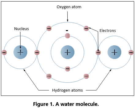
The smallest particle of matter that can exist and still retain its identity, such as water (H₂O), is called a molecule. A molecule of water is illustrated in Figure 1. Substances composed of only one type  of atom are called elements. But most substances occur in nature as compounds, that is, combinations of two    or more types of atoms. It would no longer retain the characteristics of water if it were compounded of one atom of hydrogen and two atoms of oxygen. If a drop of water is divided in two and then divided again and again until it cannot be divided any longer, it will still be water.

The Atom

The atom is considered to be the most basic building block of all matter. Atoms are composed of three sub- atomic particles. These three sub-atomic particles are: protons, neutrons, and electrons. These three particles will determine the properties of the specific atoms. Elements are substances composed of the same atoms with specific properties. Oxygen is an example of this. The main property that defines each element is the number of neutrons, protons, and electrons. Hydrogen and helium are examples of elements. Both of these elements have neutrons, protons, and electrons but differ in the number of those items. This difference alone accounts for the variations in chemical and physical properties of these two different elements. There are over a 100 known elements in the periodic table, and they are categorized according to their properties on that table. The kinetic theory of matter also states that the particles that make up the matter are always moving. Thermal expansion is considered in the kinetic theory and explains why matter contracts when it is cool and expands when it is hot, with the exception of water/ice.

Electrons, Protons, and Neutrons

At the center of the atom is the nucleus, which contains the protons and neutrons. The protons are positively charged particles, and the neutrons are a neutrally charged particle. The neutron has approximately the same mass as the proton. The third particle of the atom is the electron that is a negatively charged particle with a very small mass compared to the proton. The proton’s mass is approximately 1,837 times greater than the electron. Due to the proton and the neutron location in the central portion of the atom (nucleus) and the electron’s position at the distant periphery of the atom, it is the electron that undergoes the change during chemical reactions. Since a proton weighs approximately 1,845 times as much as an electron, the number of protons and neutrons in its nucleus deter- mines the overall weight of an atom. The weight of an electron is not considered in determining the weight of an atom. Indeed, the nature of electricity cannot be defined clearly because it is not certain whether the electron is a negative charge with no mass (weight) or a particle of matter with a negative charge.

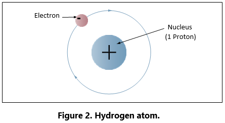
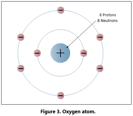
Hydrogen represents the simplest form of an atom, as shown in Figure 2. At the nucleus of the hydrogen atom is one proton and at the outer shell is one orbiting electron. At a more complex level is the oxygen atom, as shown in Figure 3, which has eight electrons in two shells orbiting the nucleus with  eight protons and eight neutrons. When the total positive charge of the protons in the nucleus equals the total negative charge of the electrons in orbit around the nucleus, the atom is said to have a neutral charge.

Electron Shells and Energy Levels

Electrons require a certain amount of energy to stay in an orbit. This particular quantity is called the electron’s energy level. By its motion alone, the electron possesses kinetic energy, while the electron’s position in orbit determines its potential energy. The total energy of an electron is the main factor, which determines the radius of the electrons orbit.

Electrons of an atom will appear only at certain definite energy levels (shells). The spacing between energy levels is such that when the chemical properties of the various elements are cataloged, it is convenient to group several closely spaced permissible energy levels together into electron shells. The maximum number of electrons that can be contained in any shell or sub-shell is the same for all atoms and is defined as Electron Capacity = 2n2. In this equation n represents the energy level in question. The first shell can only contain two electrons; the second shell can only contain eight electrons; the third, 18 and so on until we reach the seventh shell for the heaviest atoms, which have six energy levels. Because the innermost shell is the lowest energy level, the shell begins to fill up from the shell closest to the nucleus and fill outward as the atomic number of the element increases. However, an energy level does not need to be completely filled before electrons begin to fill the next level. The Periodic Table of Elements should be checked to determine an element’s electron configuration.

Valence Electrons

Valence is the number of chemical bonds an atom can form. Valence electrons are electrons that can participate in chemical bonds with other atoms. The number of electrons in the outermost shell of the atom is the determining factor in its valence. Therefore, the electrons contained in this shell are called valence electrons.

Ions

Ionization is the process by which an atom loses or gains electrons. Dislodging an electron from an atom will cause the atom to become positively charged. This net positively charged atom is called a positive ion or a cation. An atom that has gained an extra number of electrons is negatively charged and is called a negative ion or an anion. When atoms are neutral, the positively charged proton and the negatively charged electron are equal.

Free Electrons

Valence electrons are found drifting midway between two nuclei. Some electrons are more tightly bound  to the nucleus of their atom than others and are positioned in a shell or sphere closer to the nucleus, while others are more loosely bound and orbit at a greater distance from the nucleus. These outermost electrons are called “free” electrons because they can be easily dislodged from the positive attraction of the protons in the nucleus. Once freed from the atom, the electron can then travel from atom to atom, becoming the flow of electrons commonly called current in a practical electrical circuit.

Electron Movement

The valence of an atom determines its ability to gain or lose an electron, which ultimately determines the chemical and electrical properties of the atom. These properties can be categorized as being a conductor, semiconductor or insulator, depending on the ability of the material to produce free electrons. When a material has a large number of free electrons available, a greater current can be conducted in the material.

Conductors

Elements such as gold, copper and silver possess many free electrons and make good conductors. The atoms in these materials have a few loosely bound electrons in their outer orbits. Energy in the form of heat can cause these electrons in the outer orbit to break loose and drift throughout the material. Copper and silver have one electron in their outer orbits. At room temperature, a piece of silver wire will have billions of free electrons.

Insulators

These are materials that do not conduct electrical cur- rent very well or not at all. Good examples of these are: glass, ceramic, and plastic. Under normal conditions, atoms in these materials do not produce free electrons. The absence of the free electrons means that electrical current cannot be conducted through the material. Only when the material is in an extremely strong electrical field will the outer electrons be dislodged. This action is called breakdown and usually causes physical damage to the insulator.

Semiconductors

This material falls in between the characteristics of conductors and insulators, in that they are not good at conducting or insulating. Silicon and germanium are the most widely used semiconductor materials. For a more detailed explanation on this topic refer to Page 101 in this chapter.

Metric Based Prefixes Used for Electrical Calculations

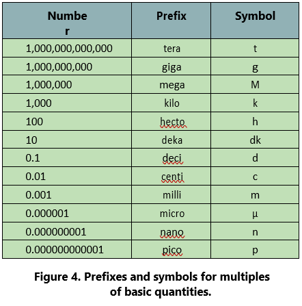
In any system of measurements, a single set of units is usually not sufficient for all the computations involved in electrical repair and maintenance. Small distances, for example, can usually be measured in inches, but larger distances are more meaningfully expressed in feet, yards, or miles. Since electrical values often vary from numbers that are a millionth part of a basic unit of measurement to very large values, it is often necessary to use a wide range of numbers to represent the values of such units as volts, amperes, or ohms. A series of prefixes which appear with the name of the unit have been devised for the various multiples or submultiples of the basic units. There are 12 of these prefixes, which are also known as conversion factors. Four of the most commonly used prefixes used in electrical work with a short definition of each are as follows:

Mega (M) means one million (1,000,000).

Kilo (k) means one thousand (1,000).

Milli (m) means one-thousandth (¹⁄1,000).

Micro (μ) means one-millionth (¹⁄1,000,000).

One of the most extensively used conversion factors, kilo, can be used to explain the use of prefixes with basic units of measurement. Kilo means 1,000, and when used with volts, is expressed as kilovolt, meaning 1,000 volts. The symbol for kilo is the letter “k”. Thus, 1,000 volts is one kilovolt or 1kV. Conversely, one volt would equal one-thousandth of a kV, or ¹⁄1,000

kV. This could also be written 0.001 kV.

Similarly, the word “milli” means one-thousandth, and thus, 1 millivolt equals one-thousandth (¹⁄1000)  of a volt.

Figure 4 contains a complete list of the multiples used to express electrical quantities, together with the prefixes and symbols used to represent each number.

Chapter: 2 Static Electricity

Electricity is often described as being either static or dynamic. The difference between the two is based simply on whether the electrons are at rest (static) or in motion (dynamic). Static electricity is a build up of an electrical charge on the surface of an object. It is considered “static” due to the fact that there is no cur- rent flowing as in AC or DC electricity. Static electricity is usually caused when non-conductive materials such as rubber, plastic or glass are rubbed together, causing a transfer of electrons, which then results in an imbalance of charges between the two materials. The fact that there is an imbalance of charges between the two materials means that the objects will exhibit an attractive or repulsive force.

Attractive and Repulsive Forces

One of the most fundamental laws of static electricity, as well as magnetics, deals with attraction and repulsion. Like charges repel each other and unlike charges attract each other. All electrons possess a negative charge and as such will repel each other. Similarly, all protons possess a positive charge and as such will repel each other. Electrons (negative) and protons (positive) are opposite in their charge and will attract each other.

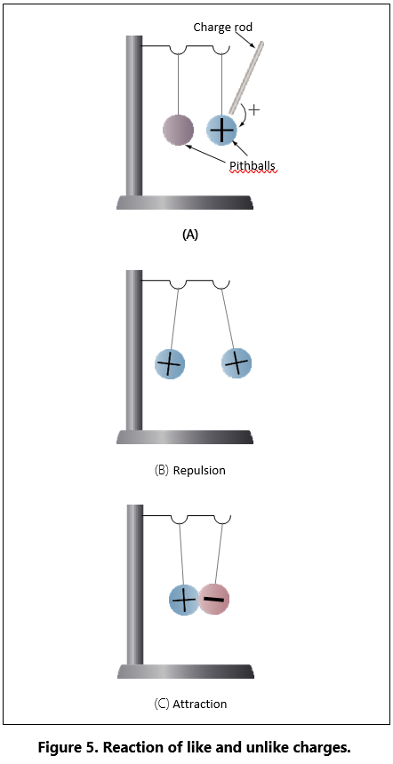
For example, if two pith balls are suspended, as shown in Figure 5, and each ball is touched with the charged glass rod, some of the charge from the rod is transferred to the balls. The balls now have similar charges and, consequently, repel each other as  shown in part B of Figure 5. If a plastic rod is rubbed with fur, it becomes negatively charged and the fur is positively charged. By touching each ball with these differently charged sources, the balls obtain opposite charges and attract each other as shown in part C of Figure 5.

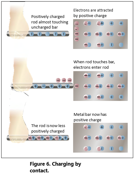
Although most objects become charged with static electricity by means of friction, a charged substance can also influence objects near it by contact. This is illustrated in Figure 6. If a positively charged rod touches an uncharged metal bar, it will draw electrons from the uncharged bar to the point of contact. Some electrons will enter the rod, leaving the metal bar with a deficiency of electrons (positively charged) and making the rod less positive than it was or, perhaps, even neutralizing its charge completely.

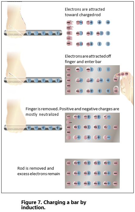
A method of charging a metal bar by induction is demonstrated in Figure 7. A positively charged rod  is brought near, but does not touch, an uncharged metal bar. Electrons in the metal bar are attracted to the end of the bar nearest the positively charged rod, leaving a deficiency of electrons at the opposite end of the bar. If this positively charged end is touched by a neutral object, electrons will flow into the metal bar and neutralize the charge. The metal bar is left with an overall excess of electrons.

Electrostatic Field

Afield of force exists around a charged body. This field is an electrostatic field (sometimes called a dielectric field) and is represented by lines extending in all directions from the charged body and terminating where there is an equal and opposite charge.

To explain the action of an electrostatic field, lines are used to represent the direction and intensity of the electric field of force. As illustrated in Figure 8, the intensity of the field is indicated by the number of lines per unit area, and the direction is shown by arrowheads on the lines pointing in the direction in which a small test charge would move or tend to move if acted upon by the field of force.

Either a positive or negative test charge can be used, but it has been arbitrarily agreed that a small positive charge will always be used in determining the direction of the field. Thus, the direction of the field around a positive charge is always away from the charge, as shown in Figure 8, because a positive test charge would be repelled. On the other hand, the direction of the lines about a negative charge is toward the charge, since a positive test charge is attracted toward it.

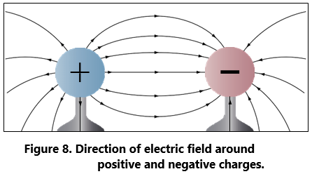
Figure 9 illustrates the field around bodies having like charges. Positive charges are shown, but regard- less of the type of charge, the lines of force would repel each other if the charges were alike. The lines terminate on material objects and always extend from a positive charge to a negative charge. These lines are imaginary lines used to show the direction a real force takes.

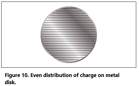
It is important to know how a charge is distributed on an object. Figure 1-10 shows a small metal disk on which a concentrated negative charge has been placed. By using an electrostatic detector, it can be shown that the charge is spread evenly over the entire surface of the disk. Since the metal disk provides uniform resistance everywhere on its surface, the mutual repulsion of electrons will result in an even distribution over the entire surface.

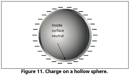
Another example, shown in Figure 11, is the charge on a hollow sphere. Although the sphere is made of conducting material, the charge is evenly distributed over the outside surface. The inner surface is completely neutral. This phenomenon is used to safeguard operating personnel of the large Van de Graaff static generators used for atom smashing. The safest area for the operators is inside the large sphere, where millions of volts are being generated.

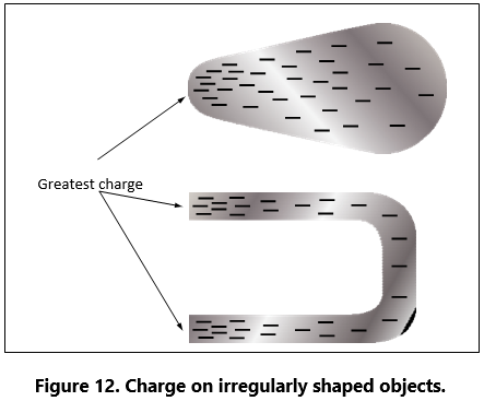
The distribution of the charge on an irregularly shaped object differs from that on a regularly shaped object. Figure 12 shows that  the  charge  on  such  objects is not evenly distributed. The greatest charge is at  the points, or areas of sharpest curvature, of the objects.

ESD Considerations

One of the most frequent causes of damage to a solid-state component or integrated circuits is the electrostatic discharge (ESD) from the human body when one of these devices is handled. Careless handling  of line replaceable units (LRUs), circuit cards, and discrete components can cause unnecessarily time consuming and expensive repairs. This damage can occur if a technician touches the mating pins for a card or box. Other sources for ESD can be the top of a toolbox that is covered with a carpet. Damage can be avoided by discharging the static electricity from your body by touching the chassis of the removed box, by wearing a grounding wrist strap, and exercising good professional handling of the components in the field. This can include placing protective caps over open connectors and not placing an ESD sensitive component in an environment that will cause damage. Parts that are ESD sensitive are typically shipped in bags specially designed to protect components from electrostatic damage.

Other precautions that should be taken with working with electronic components are:

1. Always connect a ground between test equipment and circuit before attempting to inject or monitor a signal.
2. Ensure test voltages do not exceed maximum allowable voltage for the circuit components and transistors.
3. Ohmmeter ranges that require a current of more than one milliampere in the test circuit should not be used for testing transistors.
4. The heat applied to a diode or transistor, when soldering is required, should be kept to a minimum by using low-wattage soldering irons and heat- sinks.
5. Do not pry components off of a circuit board.
6. Power must be removed from a circuit before replacing a component.
7. When using test probes on equipment and the space between the test points is very close, keep the exposed portion of the leads as short as possible to prevent shorting.

Chapter: 3 Magnetism

Magnetism is defined as the property of an object to attract certain metallic substances. In general, these substances are ferrous materials; that is, materials composed of iron or iron alloys, such as soft iron, steel, and alnico. These materials, sometimes called magnetic materials, today include at least three nonferrous materials: nickel, cobalt, and gadolinium, which are magnetic to a limited degree. All other substances are considered nonmagnetic, and a few of these non- magnetic substances can be classified as diamagnetic since they are repelled by both poles of a magnet.

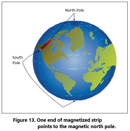
Magnetism is an invisible force, the ultimate nature of which has not been fully determined. It can best be described by the effects it produces. Examination of a simple bar magnet similar to that illustrated in Figure 13 discloses some basic characteristics of all mag- nets. If the magnet is suspended to swing freely, it will align itself with the earth’s magnetic poles. One end is labeled “N,” meaning the north seeking end or pole of the magnet. If the “N” end of a compass or magnet is referred to as north seeking rather than north, there will be no conflict in referring to the pole it seeks, which is the north magnetic pole. The opposite end of the magnet, marked “S” is the south seeking end and points to the south magnetic pole. Since the earth is a giant magnet, its poles attract the ends of the magnet. These poles are not located at the geographic poles.

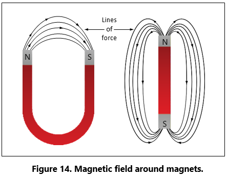
The somewhat mysterious and completely invisible force of a magnet depends on a magnetic field that surrounds the magnet as illustrated in Figure 14. This field always exists between the poles of a magnet, and will arrange itself to conform to the shape of any magnet.

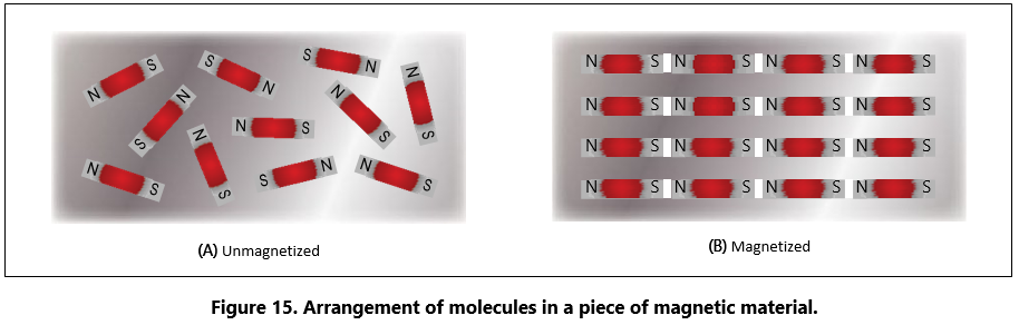
The theory that explains the action of a magnet holds that each molecule making up the iron bar is itself a tiny magnet, with both north and south poles as illustrated in Figure 15A. These molecular magnets each possess a magnetic field, but in an un-magnetized state, the molecules are arranged at random throughout the iron bar. If a magnetizing force, such as stroking with a lodestone, is applied to the un-magnetized bar, the molecular magnets rearrange themselves in line with the magnetic field of the lodestone, with all north ends of the magnets pointing in one direction and all south ends in the opposite direction. This is illustrated in Figure 15B. In such a configuration, the magnetic fields of the magnets combine to produce the total field of the magnetized bar.

When handling a magnet, avoid applying direct heat, or hammering or dropping it. Heating or sudden shock will cause misalignment of the molecules, causing the strength of a magnet to decrease. When a magnet is to be stored, devices known as “keeper bars” are installed to provide an easy path for flux lines from one pole to the other. This promotes the retention of the molecules in their north-south alignment.

The presence of the magnetic force or field around a magnet can best be demonstrated by the experiment illustrated in Figure 16. A sheet of transparent material, such as glass or Lucite™, is placed over a bar magnet and iron filings are sprinkled slowly on this transparent shield. If the glass or Lucite is tapped lightly, the iron filings will arrange themselves in a definite pattern around the bar, forming a series of lines from the north to south end of the bar to indicate the pattern of the magnetic field.

As shown, the field of a magnet is made up of many individual forces that appear as lines in the iron filing demonstration. Although they are not “lines” in the ordinary sense, this word is used to describe the individual nature of the separate forces making up the entire magnetic field. These lines of force are also referred to as magnetic flux.

They are separate and individual forces, since one line will never cross another; indeed, they actually repel one another. They remain parallel to one another and resemble stretched rubber bands, since they are held in place around the bar by the internal magnetizing force of the magnet.

The demonstration with iron filings further shows that the magnetic field of a magnet is concentrated at the ends of the magnet. These areas of concentrated flux are called the north and south poles of the magnet. There is a limit to the number of lines of force that can be crowded into a magnet of a given size. When a magnetizing force is applied to a piece of magnetic material, a point is reached where no more lines of force can be induced or introduced. The material is then said to be saturated.

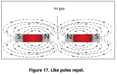
The characteristics of the magnetic flux can be demonstrated by tracing the flux patterns of two bar magnets with like poles together, as shown in Figure 17. The two like poles repel  one  another  because the lines of force will not cross each other. As the arrows on the individual lines indicate, the lines turn aside as the two like poles are brought near each other and travel in a path parallel to each other. Lines moving in this man- ner repel each other, causing the magnets as a whole to repel each other.

As the unlike poles are brought near each other, the lines of force rearrange their paths and most of the flux leaving the north pole of one magnet enters the south pole of the other. The tendency of lines of force to repel each other is indicated by the bulging of the flux in the air gap between the two magnets.By reversing the position of one of the magnets, the attraction of unlike poles can be demonstrated, as shown in Figure 18.

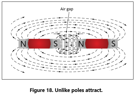
As the unlike poles are brought near each other, the lines of force rearrange their paths and most of the flux leaving the north pole of one magnet enters the south pole of the other. The tendency of lines of force to repel each other is indicated by the bulging of the flux in the air gap between the two magnets.

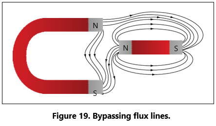
To further demonstrate that lines of force will not cross one another, a bar magnet and a horseshoe magnet can be positioned to display a magnetic field similar to that of Figure 19. The magnetic fields of the two magnets do not combine, but are rearranged into a distorted flux pattern.

The two bar magnets may be held in the hands and the north poles brought near each other to demonstrate the force of repulsion between like poles. In a similar manner, the two south poles can demonstrate this force. The force of attraction between unlike poles can be felt by bringing a south and a north  end  together.  These experiments are illustrated in Figure 20.

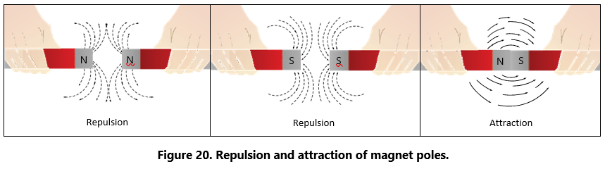
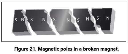
Figure 21 illustrates another characteristic of mag- nets. If the bar magnet is cut or broken into pieces, each piece immediately becomes a magnet itself, with a north and south pole. This feature supports the theory that each molecule is a magnet, since each successive division of the magnet produces still more magnets.

Since the magnetic lines of force form a continuous loop, they form a magnetic circuit. It is impossible to say where in the magnet they originate or start. Arbitrarily, it is assumed that all lines of force leave the north pole of any magnet and enter at the south pole.

There is no known insulator for magnetic flux, or lines of force, since they will pass through all materials. However, they will pass through some materials more easily than others.

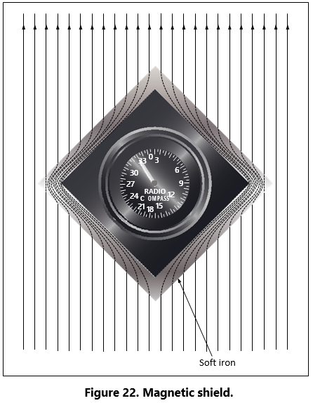
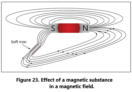
Thus it is possible to shield items such as instruments from the effects of the flux by surrounding them with a material that offers an easier path for the lines of force. Figure 22 shows an instrument surrounded by a path of soft iron, which offers very little opposition to magnetic flux. The lines of force take the easier path, the path of greater permeability, and are guided away from the instrument.

Materials such as soft iron and other ferrous metals are said to have a high permeability, the measure of the ease with which magnetic flux can penetrate a material. The permeability scale is based on a perfect vacuum with a rating of one. Air and other nonmagnetic materials are so close to this that they are also considered to have a rating of one. The nonferrous metals with a permeability greater than one, such as nickel and cobalt, are called para-magnetic. The term ferromagnetic is applied to iron and its alloys, which have by far the greatest permeability. Any substance, such as bismuth, having a permeability of less than one, is considered dia-magnetic.

Reluctance, the measure of opposition to the lines   of force through a material, can be compared to the resistance of an electrical circuit. The reluctance of soft iron, for instance, is much lower than that of air. Figure 23 demonstrates that a piece of soft iron placed near the field of a magnet can distort the lines of force, which follow the path of lowest reluctance through the soft iron.

The magnetic circuit can be compared in many respects to an electrical circuit. The magnetomotive force, causing lines of force in the magnetic circuit, can be compared to the electromotive force or electrical pres- sure of an electrical circuit. The magnetomotive force is measured in gilberts, symbolized by the capital letter “F.” The symbol for the intensity of the lines of force, or flux, is the Greek letter phi, and the unit of field intensity is the gauss. An individual line of force, called a maxwell, in an area of one square centimeter produces a field intensity of one gauss. Usingreluctance rather than permeability, the law for magnetic circuits can be stated: a magnetomotive force of one gilbert will cause one maxwell, or line of force, to be set up in a material when the reluctance of the material is one.

Types of Magnets

Magnets are either natural or artificial. Since naturally occurring magnets or lodestones have no practical use, all magnets considered in this study are artificial or manmade. Artificialmagnets can be further classified as permanent magnets, which retain their magnetism long after the magnetizing force has been removed, and temporary magnets, which quickly lose most of their magnetism when the external magnetizing force is removed.

Modern permanent magnets are made of special alloys that have been found through research to create increas- ingly better magnets. The most common categories of magnet materials are made out of Aluminum-Nickel- Cobalt (Alnicos), Strontium-Iron (Ferrites, also known as Ceramics), Neodymium-Iron-Boron (Neo magnets), and Samarium-Cobalt. Alnico, an alloy of iron, alumi- num, nickel and cobalt, and is considered one of the very best. Others with excellent magnetic qualities are alloys such as Remalloy™ and Permendur™.

The ability of a magnet to hold its magnetism varies greatly with the type of metal and is known as retentivity. Magnets made of soft iron are very easily magnetized but quickly lose most of their magnetism when the external magnetizing force is removed. The small amount of magnetism remaining, called residual magnetism, is of great importance in such electrical applications as generator operation.

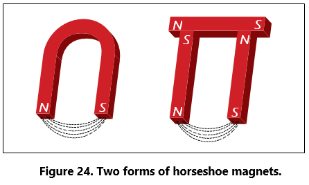
Horseshoe magnets are commonly manufactured in two forms. [Figure 24] The most common type is made from a long bar curved into a horseshoe shape, while a variation of this type consists of two bars connected by a third bar, or yoke.

Magnets can be made in many different shapes, such as balls, cylinders, or disks. One special type of mag- net is the ring magnet, or Gramme ring, often used in instruments. This is a closed loop magnet, similar to the type used in transformer cores, and is the only type that has no poles.

Sometimes special applications require that the field of force lie through the thickness rather than the length of a piece of metal. Such magnets are called flat magnets and are used as pole pieces in generators and motors.

Electromagnetism

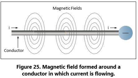
In 1820, the Danish physicist, Hans Christian Oersted, discovered that the needle of a compass brought near a current carrying conductor would be deflected. When the current flow stopped, the compass needle returned to its original position. This important discovery demonstrated a relationship between electricity and magnetism that led to the electromagnet and to many of the inventions on which modern industry is based.

Oersted discovered that the magnetic field had no connection with the conductor in which the electrons were flowing, because the conductor was made of nonmagnetic copper. The electrons moving through the wire created the magnetic field around the conductor. Since a magnetic field accompanies a charged particle, the greater the current flow, and the greater the magnetic field. Figure 25 illustrates the magnetic field around a current carrying wire. A series of concentric circles around the conductor represent the field, which if all the lines were shown would appear more as a continuous cylinder of such circles around the conductor.

As long as current flows in the conductor, the lines of force remain around it. [Figure 26] If a small cur- rent flows through the conductor, there will be a line of force extending out to circle A.If the current flow is increased, the line of force will increase in size to circle B, and a further increase in current will expand it to circle C. As the original line (circle) of force expands from circle A to B, a new line of force will appear at circle A.Asthe current flow increases, the number of circles of force increases, expanding the outer circles farther from the surface of the current carrying conductor.

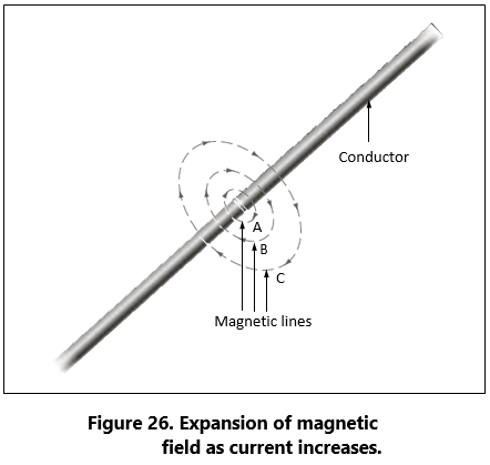
If the current flow is a steady non-varying direct current, the magnetic field remains stationary. When the current stops, the magnetic field collapses and the magnetism around the conductor disappears.

A compass needle is used to demonstrate the direction of the magnetic field around a current carrying conductor. Figure 27 View A shows a compass needle positioned at right angles to, and approximately one inch from, a current carrying conductor. If no current were flowing, the north seeking end of the compass needle would point toward the earth’s magnetic pole. When current flows, the needle lines itself up at right angles to a radius drawn from the conductor. Since the compass needle is a small magnet, with lines of force extending from south to north inside the metal, it will turn until the direction of these lines agrees with the direction of the lines of force around the conductor. As the compass needle is moved around the conductor, it will maintain itself in a position at right angles to the conductor, indicating that the magnetic field around a current carrying conductor is circular. As shown in View B of Figure 27, when the direction of current flow through the conductor is reversed, the compass needle will point in the opposite direction, indicating the magnetic field has reversed its direction.

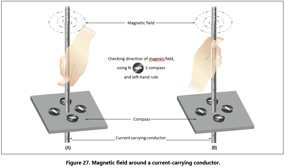
A method used to determine the direction of the lines of force when the direction of the current flow is known, is shown in Figure 28. If the conductor is grasped in the left hand, with the thumb pointing in the direction of current flow, the fingers will be wrapped around the conductor in the same direction as the lines of the magnetic field. This is called the left-hand rule.

Although it has been stated that the lines of force have direction, this should not be construed to mean that the lines have motion in a circular direction around the conductor. Although the lines of force tend to act in a clockwise or counterclockwise direction, they are not revolving around the conductor.

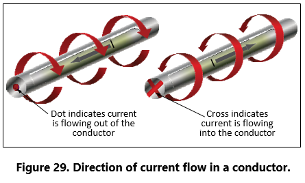
Since current flows from negative to positive, many illustrations indicate current direction with a dot symbol on the end of the conductor when the electrons are flowing toward and a plus sign when the current is flowing away from the observer. [Figure 29]

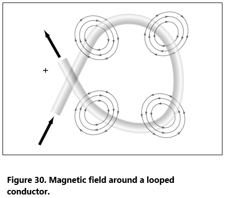
When a wire is bent into a loop and an electric cur- rent flows through it, the left-hand rule remains valid. [Figure 30]

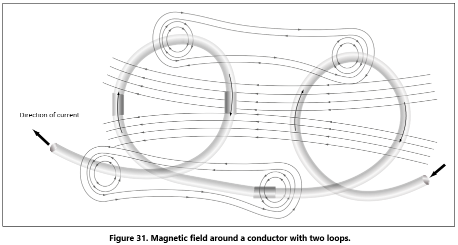
If the wire is coiled into two loops, many of the lines of force become large enough to include both loops. Lines of force go through the loops in the same direction, circle around the outside of the two coils, and come in at the opposite end. [Figure 31]

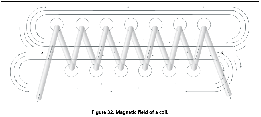
When a wire contains many such loops, it is called   a coil. The lines of force form a pattern through all the loops, causing a high concentration of flux lines through the center of the coil. [Figure 32]

In a coil made from loops of a conductor, many of the lines of force are dissipated between the loops of the coil. By placing a soft iron bar inside the coil, the lines of force will be concentrated in the center of the coil, since soft iron has a greater permeability than air.  [Figure 33] This combination of an iron core in a coil of wire loops, or turns, is called an electromagnet, since the poles (ends) of the coil possess the characteristics of a bar magnet.

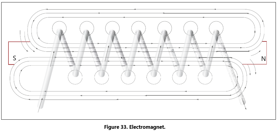
The addition of the soft iron core does two things for the current carrying coil. First, the magnetic flux is increased, and second, the flux lines are more highly concentrated.

When direct current flows through the coil, the core will become magnetized with the same polarity (location of north and south poles) as the coil would have without the core. If the current is reversed, the polarity will also be reversed.

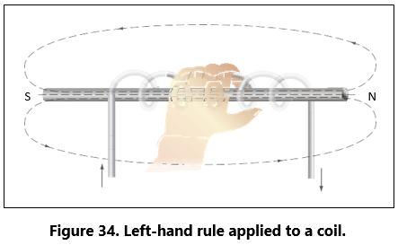
The polarity of the electromagnet is determined by the left-hand rule in the same manner as the polarity of the coil without the core was determined. If the coil is grasped in the left hand in such a manner that the fingers curve around the coil in the direction of electron flow (minus to plus), the thumb will point in the direction of the north pole. [Figure 34]

The strength of the magnetic field of the electromagnet can be increased by either increasing the flow of cur- rent or the number of loops in the wire. Doubling the current flow approximately doubles the strength of the field, and in a similar manner, doubling the number of loops approximately doubles magnetic field strength. Finally, the type metal in the core is a factor in the field strength of the electromagnet.

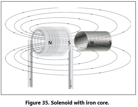
A soft iron bar is attracted to either pole of a permanent magnet and, likewise, is attracted by a current carrying coil. The lines of force extend through the soft iron, magnetizing it by induction and pulling the iron bar toward the coil. If the bar is free to move, it will be drawn into the coil to a position near the center where the field is strongest. [Figure 35]

Electromagnets are used in electrical instruments, motors, generators, relays, and other devices. Some electromagnetic devices operate on the principle that an iron core held away from the center of a coil will be rapidly pulled into a center position when the coil is energized. This principle is used in the solenoid, also called solenoid switch or relay, in which the iron core is spring-loaded off center and moves to complete a circuit when the coil is energized.

Chapter: 4 Conventional Flow and Electron Flow

Today’s technician will find that there are two competing schools of thought and analytical practices regarding the flow of electricity. The two are called the conventional current theory and the electron theory.

Conventional Flow

Of the two, the conventional current theory was the first to be developed and, through many years of use, this method has become ingrained in electrical texts. The theory was initially advanced by Benjamin Franklin who reasoned that current flowed out of a positive source into a negative source or an area that lacked an abundance of charge. The notation assigned to the electric charges was positive (+) for the abundance of charge and negative (−) for a lack of charge. It then seemed natural to visualize the flow of current as being from the positive (+) to the negative (−).

Electron Flow

Later discoveries were made that proved that just the opposite is true. Electron flow is what actually happens where an abundance of electrons flow out of the negative (−) source to an area that lacks electrons or the positive (+) source.

Both conventional flow and electron flow are used in industry. Many textbooks in current use employ both electron flow and conventional flow methods. From the practical standpoint of the technician, troubleshooting a system, it makes little to no difference which way current is flowing as long as it is used consistently in the analysis.

Electromotive Force (Voltage)

Unlike current, which is easy to visualize as a flow, voltage is a variable that is determined between two points. Often we refer to voltage as a value across two points. It is the electromotive force (emf) or the push or pressure felt in a conductor that ultimately moves the electrons in a flow. The symbol for emf is the capital letter “E.”

Across the terminals  of  the  typical  battery,  voltage can be measured as the potential difference of 12 volts or 24 volts. That is to say that between the two terminal posts of the battery, there is an electromotive force of 12 or 24 volts available to push current through a circuit. Relatively free electrons in the negative terminal will move toward the excessive number of positive charges in the positive terminal. Recall from the discussion on static electricity that like charges repel each other but opposite charges attract each other. The net result is a flow or current through a conductor. There cannot be a flow in a conductor unless there is an applied voltage from a battery, generator, or ground power unit. The potential difference, or the voltage across any two points in an electrical system, can be determined by:

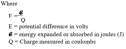
Figure 36 illustrates the flow of electrons of electric current. Two interconnected water tanks demonstrate that when a difference of pressure exists between the two tanks, water will flow until the two tanks are equal- ized. The illustration shows the level of water in tank A to be at a higher level, reading 10 psi (higher potential energy) than the water level in tank B, reading 2 psi (lower potential energy). Between the two tanks, there is 8-psi potential difference. If the valve in the intercon- necting line between the tanks is opened, water will flow from tank A into tank B until the level of water (potential energy) of both tanks is equalized.

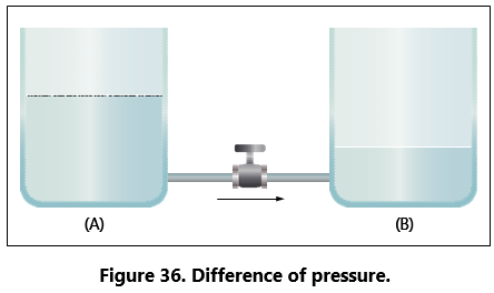
It is important to note that it was not the pressure in tank A that caused the water to flow; rather, it was the difference in pressure between tank A and tank B that caused the flow.

This comparison illustrates the principle that electrons move, when a path is available, from a point of excess electrons (higher potential energy) to a point deficient in electrons (lower potential energy). The force that causes this movement is the potential difference in electrical energy between the two points. This force is called the electrical pressure or the potential difference or the electromotive force (electron moving force).

Current

Electrons in motion make up an electric current. This electric current is usually referred to as “current” or “current flow,” no matter how many electrons are moving. Current is a measurement of a rate at which a charge flows through some region of space or a conductor. The moving charges are the free electrons found in conductors, such as copper, silver, aluminum, and gold. The term “free electron” describes a condition in some atoms where the outer electrons are loosely bound to their parent atom. These loosely bound electrons can be easily motivated to move in a given direction when an external source, such as a battery, is applied to the circuit. These electrons are attracted to the positive terminal of the battery, while the negative terminal is the source of the electrons. The greater amount of charge moving through the conductor in a given amount of time translates into a current.

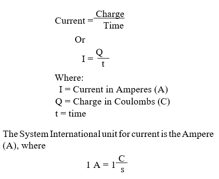
That is, 1 ampere (A) of current is equivalent to 1 coulomb (C) of charge passing through a conductor in 1 second(s). One coulomb of charge equals 6.28 billion billion electrons. The symbol used to indicate current in formulas or on schematics is the capital letter “I.”

When current flow is one direction, it is called direct current (DC). Later in the text, we will discuss the form of current that periodically oscillates back and forth within the circuit. The present discussion will only be concerned with the use of direct current.

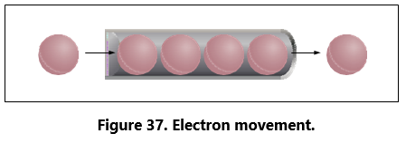
The velocity of the charge is actually an average velocity and is called drift velocity. To understand the idea of drift velocity, think of a conductor in which the charge carriers are free electrons. These electrons are always in a state of random motion similar to that of gas molecules. When a voltage is applied across the conductor, an electromotive force creates an electric field within the conductor and a current is established. The electrons do not move in a straight direction but undergo repeated collisions with other nearby atoms. These collisions usually knock other free electrons from their atoms, and these electrons move on toward the positive end of the conductor with an average velocity called the drift velocity, which is relatively a slow speed. To understand the nearly instantaneous speed of the effect of the current, it is helpful to visualize a long tube filled with steel balls as shown in Figure 37. It can be seen that a ball introduced in one end of the tube, which represents the conductor, will immediately cause a ball to be emitted at the opposite end of the tube. Thus, electric current can be viewed as instantaneous, even though it is the result of a relatively slow drift of electrons.

Ohm’s Law (Resistance)

The two fundamental properties of current and voltage are related by a third property known as resistance. In any electrical circuit, when voltage is applied to it, a current will result. The resistance of the conductor will determine the amount of current that flows under the given voltage. In most cases, the greater the cir- cuit resistance, the less the current. If the resistance is reduced, then the current will increase. This relation is linear in nature and is known as Ohm’s law.

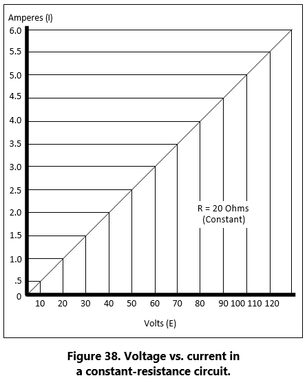
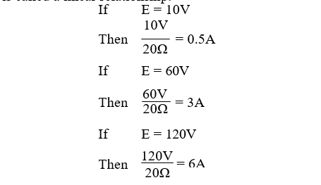
By having a linearly proportional characteristic, it is meant that if one unit in the relationship increases or decreases by a certain percentage, the other vari- ables in the relationship will increase or decrease  by the same percentage. An example would be if the voltage across a resistor is doubled, then the current through the resistor doubles. It should be added that this relationship is true only if the resistance in the circuit remains constant. For it can be seen that if the resistance changes, current also changes.  A  graph of this relationship is shown in Figure 38, which uses a constant resistance of 20Ω. The relationship between voltage and current in this example shows voltage plot-ted horizontally along the X axis in values from 0 to 120 volts, and the corresponding values of current are plotted vertically in values from 0 to 6.0 amperes along the Y axis. A straight line drawn through all the points where the voltage and current lines meet represents the equation I = ^E⁄20 and is called a linear relationship.

Ohm’s law may be expressed as an equation, as follows:

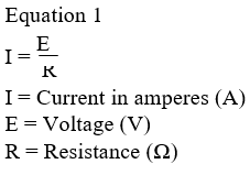
Where I is current in amperes, E is the potential difference measured in volts, and R is the resistance measured in ohms. If any two of these circuit quantities are known, the third may be found by simple algebraic transposition. With this equation, we can calculate cur- rent in a circuit if the voltage and resistance are known. This same formula can be used to calculate voltage. By multiplying both sides of the equation 1 by R, we get an equivalent form of Ohm’s law, which is:

Finally, if we divide equation 2 by I, we will solve for resistance,

All three formulas presented in this section are equivalent to each other and are simply different ways of expressing Ohm’s law.

The various equations, which may be derived by trans- posing the basic law, can be easily obtained by using the triangles in Figure 39.

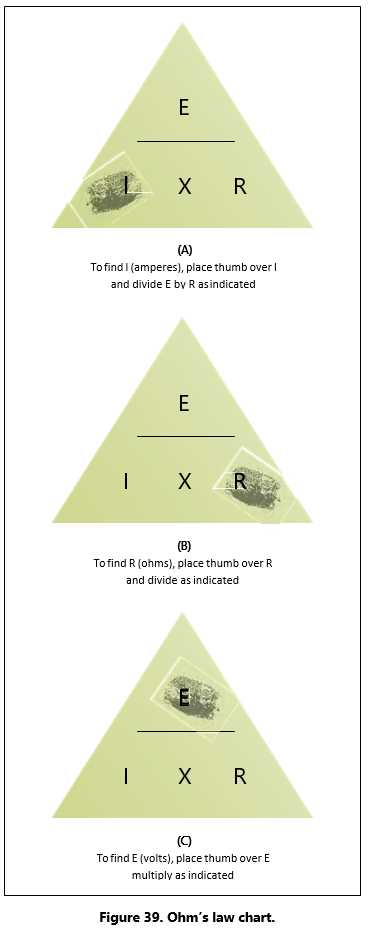
The triangles containing E, R, and I are divided into two parts, with E above the line and I × R below it. To determine an unknown circuit quantity when the other two are known, cover the unknown quantity with a Then 20Ω = 0.5A thumb. The location of the remaining uncovered letters in the triangle will indicate the mathematical operation

If E = 60V to be performed. For example, to find I, refer to Then 60V 20Ω = 3A Figure 39A, and cover I with the thumb. The uncovered letters indicate that E is to be divided by If E = 120V R, or I = ^E⁄R. To find R, refer to Figure 39B, and cover R with the thumb. The result indicates that E is to be Then 120V = 6A 20Ω divided by I, or R = ^E⁄I. To find E, refer to Figure 39C, and cover E with the thumb. The result  indicates I is to be multiplied by R, or E = I × R.

This chart is useful when learning to use Ohm’s law. It should be used to supplement the beginner’s knowledge of the algebraic method.

Resistance of a Conductor

While wire of any size or resistance value may be  used, the word “conductor” usually refers to materials that offer low resistance to current flow, and the word “insulator” describes materials that offer high resistance to current. There is no distinct dividing line between conductors and insulators; under the proper conditions, all types of material conduct some cur- rent. Materials offering a resistance to current flow midway between the best conductors and the poorest conductors (insulators) are sometimes referred to as “semiconductors,” and find their greatest application in the field of transistors.

The best conductors are materials, chiefly metals, which possess a large number of free electrons; conversely, insulators are materials having few free electrons. The best conductors are silver, copper, gold, and aluminum; but some nonmetals, such as carbon and water, can be used as conductors. Materials such as rubber, glass, ceramics, and plastics are such poor conductors that they are usually used as insulators. The current flow in some of these materials is so low that it is usually considered zero. The unit used to measure resistance is called the ohm. The symbol for the ohm is the Greek letter omega (Ω). In mathematical formulas, the capital letter “R” refers to resistance. The resistance of a conductor and the voltage applied to it determine the number of amperes of current flowing through the conductor. Thus, 1 ohm of resistance will limit the current flow to 1 ampere in a conductor to which a voltage of 1 volt is applied.

Factors Affecting Resistance

1. The resistance of a metallic conductor is dependent on the type of conductor material. It has been pointed out that certain metals are commonly used as conductors because of the large number of free electrons in their outer orbits. Copper is usually considered the best available conductor material, since a copper wire of a particular diameter offers a lower resistance to current flow than an aluminum wire of the same diameter. However, aluminum is much lighter than copper, and for this reason as well as cost considerations, aluminum is often used when the weight factor is important.
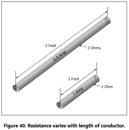
2. The resistance of a metallic conductor is directly proportional to its The longer the length of a given size of wire, the greater the resistance. Figure 40.  shows two wire conductors of different lengths. If 1 volt of electrical pressure is applied across the two ends of the conductor that is 1 foot in length and the resistance to the movement of free electrons is assumed to be 1 ohm, the current flow is limited to 1 ampere. If the same size conductor is doubled in length, the same electrons set in motion by the 1 volt applied now find twice the resistance; consequently, the current flow will be reduced by one-half.
   
3. The resistance of a metallic conductor is inversely proportional to the cross-sectional area. This area may be triangular or even square, but is usually If the cross-sectional area of a conductor is doubled, the resistance to current flow will be reduced in half. This is true because of the increased area in which an electron can move without collision or capture by an atom. Thus, the resistance varies inversely with the cross-sectional area of a conductor.
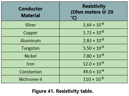
4. The fourth major factor influencing the resistance of a conductor is Although some substances, such as carbon, show a decrease in resistance as the ambient (surrounding) temperature increases, most materials used as conductors increase in resistance as temperature increases. The resistance of a few alloys, such as constantan and Manganin™, change very little as the temperature changes. The amount of increase in the resistance of a 1 ohm sample of a conductor, per degree rise in temperature above 0° Centigrade (C), the assumed standard, is called the temperature coefficient of resistance. For each metal, this is a different value; for example, for copper the value is approximately 0.00427 ohm. Thus, a copper wire having a resistance of 50 ohms at a temperature of 0 °C will have an increase in resistance of 50 he resistance of a metallic conductor is directly proportional to its The longer the length of a given size of wire, the greater the resistance. Figure 40. shows two wire conductors of different lengths. If 1 volt of electrical pressure is applied across the two ends of the conductor that is 1 foot in length and the resistance to the movement of free electrons is assumed to be 1 ohm, the current flow is limited to 1 ampere. If the same size conductor is doubled in length, the same electrons set in motion by the 1 volt applied now find twice the resistance; consequently, the current flow will be reduced by one-half. × 0.00427, or 0.214 ohm, for each degree rise   in temperature above 0 °C. The temperature coefficient of resistance must be considered where there is an appreciable change in temperature of a conductor during operation. Charts listing the temperature coefficient of resistance for different materials are available. Figure 41 shows a table for “resistivity” of some common electric conductors.
   

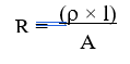
The resistance of a material is determined by four properties: material, length, area, and temperature. The first three properties are related by the following equation at T = 20 °C (room temperature):

Resistance and Its Relation to Wire Sizing

Circular Conductors (Wires/Cables)

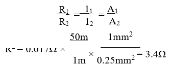
Because it is known that the resistance of a conduc- tor is directly proportional to its length, and if we are given the resistance of the unit length of wire, we can readily calculate the resistance of any length of wire of that particular material having the same diameter. Also, because it is known that the resistance of a conductor is inversely proportional to its cross-sectional area, and if we are given the resistance of a length of wire with unit cross-sectional area, we can calculate the resis- tance of a similar length of wire of the same material with any cross-sectional area. Therefore, if we know the resistance of a given conductor, we can calculate the resistance for any conductor of the same material at the same temperature. From the relationship:

It can also be written:

If we have a conductor that is 1 meter long with a cross-sectional area of 1 mm2  and has a resistance of 0.017 ohm, what is the resistance of 50m of wire from the same material but with a cross-sectional area of 0.25 mm2?

While the System International (SI) units are com- monly used in the analysis of electric circuits, electrical conductors in North America are still being manufac- tured using the foot as the unit length and the mil (one thousandth of an inch) as the unit of diameter. Before using the equation R = ^(ρ × ^l)⁄A to calculate the resis- tance of a conductor of a given AWG size, the cross- sectional area in square meters must be determined using the conversion factor 1 mil = 0.0254 mm. The most convenient unit of wire length is the foot. Using these standards, the unit of size is the mil-foot. Thus, a wire has unit size if it has a diameter of 1 mil and length of 1 foot.

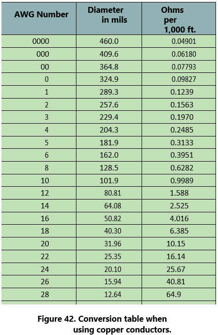
In the case of using copper conductors, we are spared the task of tedious calculations by using a table as shown in Figure 42. Note that cross-sectional dimensions listed on the table are such that each decrease of one gauge number equals a 25 percent increase in the cross-sectional area. Because of this, a decrease of three gauge numbers represents an increase in cross-sectional area of approximately a 2:1 increase. Likewise, change of ten wire gauge numbers represents a 10:1 change in cross-sectional area — also, by doubling the cross-sectional area of the conductor, the resistance is cut in half. A decrease of three wire gauge numbers cuts the resistance of the conductor of a given length in half.

Rectangular Conductors (Bus Bars)

To compute the cross-sectional area of a conductor in square mils, the length in mils of one side is squared. In the case of a rectangular conductor, the length of one side is multiplied by the length of the other. For example, a common rectangular bus bar (large, special conductor) is 3/8 inch thick and 4 inches wide. The 3/8-inch thickness may be expressed as 0.375 inch. Since 1,000 mils equal 1 inch, the width in inches can be converted to 4,000 mils. The cross-sectional area of the rectangular conductor is found by converting 0.375 to mils (375 mils × 4,000 mils = 1,500,000 square mils).

Chapter: 5 Power and Energy

Power in an Electrical Circuit

This section covers power in the DC circuit and energy consumption. Whether referring to mechanical or elec- trical systems, power is defined as the rate of energy consumption or conversion within that system — that is, the amount of energy used or converted in a given amount of time.

From the scientific discipline of physics, the fundamental expression for power is:

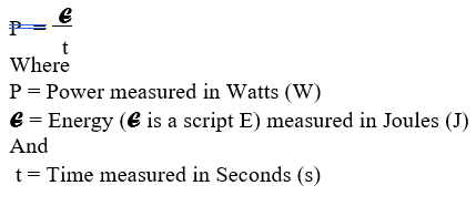
The unit measurement for power is the watt (W), which refers to a rate  of  energy  conversion of 1 joule/second. Therefore, the number of joules consumed in 1 second is equal to the number of watts. A simple example is given below.

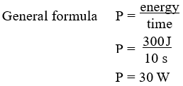
Suppose 300 J of energy is consumed in 10 seconds. What would be the power in watts?

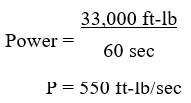
The watt is named for James Watt, the inventor of the steam engine. Watt devised an experiment to measure the power of a horse in order to find a means of measuring the mechanical power of his steam engine. One horsepower is required to move 33,000 pounds 1 foot in 1 minute. Since power is the rate of doing work, it is equivalent to the work divided by time. Stated as a formula, this is:

Electrical power can be rated in a similar manner. For example, an electric motor rated as a 1 horsepower motor requires 746 watts of electrical energy.

Power Formulas Used in the Study of Electricity

When current flows through a resistive circuit, energy is dissipated in the form of heat. Recall that voltage can be expressed in the terms of energy and charge as given in the expression:

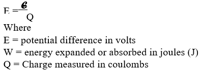
Current I, can also be expressed in terms of charge and time as given by the expression:

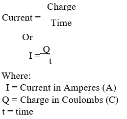
When voltage ^W⁄Q and current ^Q⁄t are multiplied, the charge Q is divided out leaving the basic expression from physics:

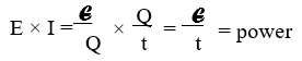
For a simple DC electrical system, power dissipation can then be given by the equation:

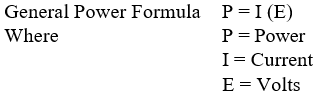
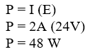
If a circuit has a known voltage of 24 volts and a current of 2 amps, then the power in the circuit will be:

Now recall Ohm’s laws which states that E = I(R). If we now substitute IR for E in the general formula, we get a formula that uses only current I and resistance R to determine the power in a circuit.

Second Form of Power Equation

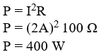
If a circuit has a known current of 2 amps and a resistance of 100 Ω, then the power in the circuit will be:

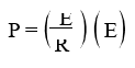
Using Ohm’s law again, which can be stated as I = ^E⁄R, we can again make a substitution such that power can be determined by knowing only the voltage (E) and resistance (R) of the circuit.

Third Form of Power Equation

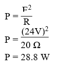
If a circuit has a known voltage of 24 volts and a resistance of 20 Ω, then the power in the circuit will be:

Power in a Series and Parallel Circuit

The total power dissipated in both a series and parallel circuit is equal to the sum of the power dissipated in each resistor in the circuit. Power is simply additive and can be stated as:

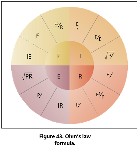
Figure 43 provides a summary of all the possible transpositions of the Ohm’s law formula and the power formula.

Energy in an Electrical Circuit

Energy is defined as the ability to do work. Because power is the rate of energy usage, power used over a span of time is actually energy consumption. If power and time are multiplied together, we will get energy.

The joule is defined as a unit of energy. There is another unit of measure which is perhaps more familiar. Because power is expressed in watts and time in seconds, a unit of energy can be called a watt-second (Ws) or more recognizable from the electric bill, a kilowatt-hour (kWh). Refer to Page 3-3 for further discussion on energy.

Sources of Electricity

Electrical energy can be produced in a number of methods. The four most common are pressure, chemical, thermal, and light.

Pressure Source

This form of electrical generation is commonly known as piezoelectric (piezo or piez taken from Greek: to press; pressure; to squeeze) is a result of the application of mechanical pressure on a dielectric or nonconducting crystal. The most common piezoelectric materials used today are crystalline quartz and Rochelle salt. However, Rochelle salt is being superseded by other materials, such as barium titanate.

The application of a mechanical stress produces an electric polarization, which is proportional to this stress. This polarization establishes a voltage across the crystal. If a circuit is connected across the crystal a flow of current can be observed when the crystal is loaded (pressure is applied). An opposite condition can occur, where an application of a voltage between certain faces of the crystal can produce a mechanical distortion. This effect is commonly referred to as the piezoelectric effect.

Piezoelectric materials are used extensively in transducers for converting a mechanical strain into an electrical signal. Such devices include microphones, phonograph pickups and vibration-sensing elements. The opposite effect, in which a mechanical output is derived from an electrical signal input, is also widely used in headphones and loudspeakers.

Chemical Source

Chemical energy can be converted into electricity; the most common form of this is the battery. A primary battery produces electricity using two different metals in a chemical solution like alkaline electrolyte, where a chemical reaction between the metals and the chemicals frees more electrons in one metal than in the other. One terminal of the battery is attached to one of the metals such as zinc; the other terminal is attached to the other metal such as manganese oxide. The end that frees more electrons develops a positive charge and the other end develops a negative charge. If a wire is attached from one end of the battery to the other, electrons flow through the wire to balance the electrical charge.

Thermal Sources

The most common source of thermal electricity found in the aviation industry comes from thermocouples. Thermocouples are widely used as temperature sen- sors. They are cheap and interchangeable, have stan- dard connectors, and can measure a wide range of temperatures. Thermocouples are pairs of dissimilar metal wires joined at least at one end, which generate a voltage between the two wires that is proportional to the temperature at the junction. This is called the Seebeck effect, in honor of Thomas Seebeck who first noticed the phenomena in 1821. It was also noticed that different metal combinations have a different voltage difference.

Thermocouples are usually pressed into service as ways to measure cylinder head temperatures and inter- turbine temperature.

Light Sources

A solar cell or a photovoltaic cell is a device that con- verts light energy into electricity. Fundamentally, the device contains certain chemical elements that when exposed to light energy, they release electrons.

Photons in sunlight are taken in by the solar panel or cell, where they are then absorbed by semiconducting materials, such as silicon. Electrons in the cell are broken loose from their atoms, allowing them to flow through the material to produce electricity. The comple- mentary positive charges that are also created are called holes (absence of electron) and flow in the direction opposite of the electrons in a silicon solar panel.

Solar cells have many applications and have his- torically been used in earth orbiting satellites or space probes, handheld calculators, and wrist watches.

Schematic Representation of Electrical Components

The schematic is the most common place where the technician will find electronic symbols. The schematic is a diagram that depicts the interconnection and logic of an electronic or electrical circuit. Many symbols are employed for use in the schematic drawings, blueprints, and illustrations. This section briefly outlines some of the more common symbols and explains how to interpret them.

Conductors

The schematic depiction of a conductor is simple enough. This is generally shown as a solid line. How- ever, the line types may vary depending on who drew the schematics and what exactly the line represents. While the solid line is used to depict the wire or con- ductor, schematics used for modifications can also use other line types such as a dashed to represent “existing” wires prior to modification and solid lines for “new” wires.

There are two methods employed to show wire cross-overs and wire connections. Figure 44 shows the two methods of drawing wires that cross, version A and version B. Figure 45 shows the two methods for drawing wire that connect version A and version B. If version A in Figure 44 is used to depict crossovers, then version A for wire connections in Figure 45 will be used. The same can then be said about the use of version B methods. The technician will encounter both in common use.

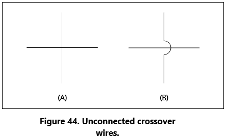
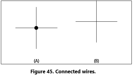
Figure 46 shows a few examples of the more common wire types that the technician will encounter in schematics. They are the single wire, single shielded, shielded twisted pair or double and the shielded triple. This is not an exhaustive list of wire types but a fair representation of how they are depicted. Figure 46 also shows the wires having a wire number. These are shown for the sake of illustration and will vary from one installation agency to another. For further understanding of a wire numbering system, consult the appropriate wiring guide published by the agency that drew the prints. Regardless of the specifics of the wire numbering system, organizations that exercise professional wiring practices will have the installed wire marked in some manner. This will be an aid to the technician who has to troubleshoot or modify the system at a later date.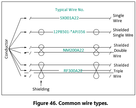 

Chapter: 6 Types of Resistors

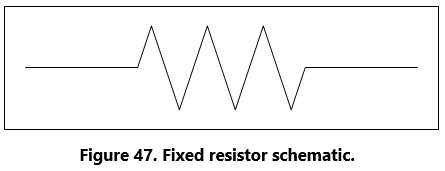
Fixed Resistor

Figure 47 is a schematic representation of a fixed resistor. Fixed resistors have built into the design a means of opposing current. The general use of a resis- tor in a circuit is to limit the amount of current flow. There are a number of methods used in construction and sizing of a resistor that control properties such as resistance value, the precision of the resistance value, and the ability to dissipate heat. While in some appli- cations the purpose of the resistive element is used to generate heat, such as in propeller anti-ice boots, heat typically is the unwanted loss of energy.

Carbon Composition

The carbon composed resistor is constructed from a mixture of finely grouped carbon/graphite, an insula- tion material for filler, and a substance for binding the material together. The amount of graphite in relation to the insulation material will determine the ohmic or resistive value of the resistor. This mixture is compressed into a rod, which is then fitted with axial leads or “pigtails.” The finished product is then sealed in an insulating coating for isolation and physi- cal protection.

There are other types of fixed resistors in common use.

Included in this group are:

• Carbon film
• Metal oxide
• Metal film
• Metal glaze

The construction of a film resistor is accomplished by depositing a resistive material evenly on a ceramic rod. This resistive material can be graphite for the car- bon film resistor, nickel chromium for the metal film resistor, metal and glass for the metal glaze resistor and last, metal and an insulating oxide for the metal oxide resistor.

Resistor Ratings

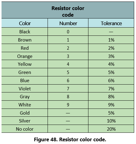
It is very difficult to manufacture a resistor to an exact standard of ohmic values. Fortunately, most circuit requirements are not extremely critical. For many uses, the actual resistance in ohms can be 20 percent higher or lower than the value marked on the resistor without causing difficulty. The percentage variation between the marked value and the actual value of a resistor   is known as the “tolerance” of a resistor. A resistor coded for a 5 percent tolerance will not be more than 5 percent higher or lower than the value indicated by the color code.

The resistor color code is made up of a group of colors, numbers, and tolerance values. Each color is repre- sented by a number, and in most cases, by a tolerance value. [Figure 48]

When the color code is used with the end-to-center band marking system, the resistor is normally marked with bands of color at one end of the resistor. The body or base color of the resistor has nothing to do with the color code, and in no way indicates a resistance value. To prevent confusion, this body will never be the same color as any of the bands indicating resistance value.

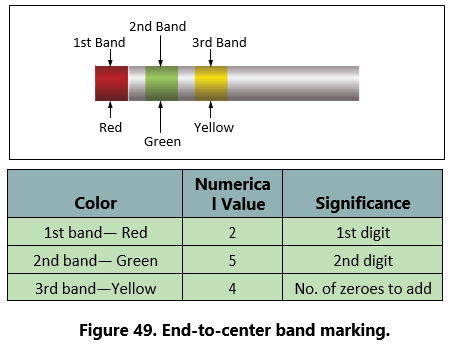
When the end-to-center band marking system is used, either three or four bands will mark the resistor.

1. The first color band (nearest the end of the resistor) will indicate the first digit in the numerical resistance value. This band will never be gold or silver in
2. The second color band will always indicate the second digit of ohmic value. It will never be gold or silver in color. [Figure 49]
3. The third color band indicates the number of zeros to be added to the two digits derived from the first and second bands, except in the following two cases.
   

(a) If the third band is gold in color, the first two digits must be multiplied by 10 percent.

(b) If the third band is silver in color, the first two digits must be multiplied by 1 percent.

4. If there is a fourth color band, it is used as a multiplier for percentage of tolerance, as indicated in the color code chart in Figure 48. If there is no fourth band, the tolerance is understood to be 20

Figure 49 provides an example,  which  illustrates the rules for reading the resistance value of a resistor marked with the end-to-center band system. This resistor is marked with three bands of color, which must be read from the end toward the center.

There is no fourth color band; therefore, the tolerance is understood to be 20 percent. 20 percent of 250,000 Ω, equals 50,000 Ω.

Since the 20 percent tolerance is plus or minus,

Maximum resistance
= 250,000 Ω + 50,000 Ω
= 300,000 Ω
Minimum resistance
= 250,000 Ω − 50,000 Ω
= 200,000 Ω

The following paragraphs provide a few extra examples of resistor color band decoding. Figure 50 contains a resistor with another set of colors. This resistor code should be read as follows:

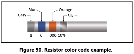
The resistance of this resistor is 86,000 ± 10 percent ohms. The maximum resistance is 94,600 ohms, and the minimum resistance is 77,400 ohms.

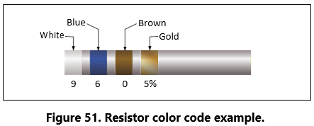
As another example, the resistance of the resistor in Figure 51 is 960 ± 5 percent ohms. The maximum resistance is 1,008 ohms, and the minimum resistance is 912 ohms.

Sometimes circuit considerations dictate that the tol- erance must be smaller than 20 percent. Figure 52 shows an example of a resistor with a 2 percent toler- ance. The resistance value of this resistor is 2,500 ± 2 percent ohms. The maximum resistance is 2,550 ohms, and the minimum resistance is 2,450 ohms.

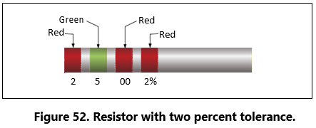
Figure 53 contains an example of a resistor with a black third color band. The color code value of black is zero, and the third band indicates the number of zeros to be added to the first two digits.

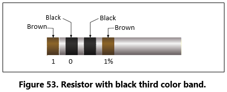
In this case, a zero number of zeros must be added to the first two digits; therefore, no zeros are added. Thus, the resistance value is 10 ± 1 percent ohms. The maximum resistance is 10.1 ohms, and the minimum resistance is 9.9 ohms. There are two exceptions to the rule stating the third color band indicates the number of zeros. The first of these exceptions is illustrated in Figure 54 When the third band is gold in color, it indicates that the first two digits must be multiplied by 10 percent. The value of this resistor in this case is:

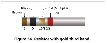
10 × 0.10 ± 2% = 1 = 0.02 ohms

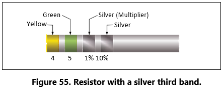
When the third band is silver, as is the case in Figure 55, the first two digits must be multiplied by 1 percent. The value of the resistor is 0.45 ± 10  percent ohms.

Wire-Wound

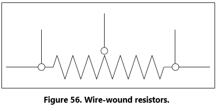
Wire-wound resistors typically control large  amounts of current and have high power ratings. Resistors of this type are constructed by winding a resistance wire around an insulating rod, usually made of porcelain. The windings are then coated with an insulation mate-rial for physical protection and heat conduction. Both ends of the windings are then connected to terminals, which are used to connect the resistor to a circuit. [Figure 56]

A wire-wound resistor with tap is a special type of fixed resistor that can be adjusted. These adjustments can be made by moving a slide bar tap or by moving the tap to a preset incremental position. While the tap may be adjustable, the adjustments are usually set at the time of installation to a specific value and then operated in service as a fixed resistor. Another type of wire-wound resistor is that constructed of Manganin wire, used where high precision is needed.

Variable Resistors

Variable resistors are constructed so that the resistive value can be changed easily. This adjustment can be manual or automatic, and the adjustments can be made while the system that it is connected to is in operation. There are two basic types of manual adjustors. One is the rheostat and the second is the potentiometer.

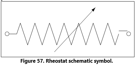
Rheostat

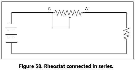
The schematic symbol for the rheostat is shown in Fig-ure 57. A rheostat is a variable resistor used to vary the amount of current flowing in a circuit. Figure 58 shows a rheostat connected in series with an ordinary resistance in a series circuit. As the slider arm moves from point A to B, the amount of  rheostat resistance (AB) is increased. Since the rheostat resistance and the fixed resistance are in series, the total resistance in the circuit also increases, and the current in the circuit decreases. On the other hand, if the slider arm is moved toward  point A, the total resistance decreases and the  current in the circuit increases.

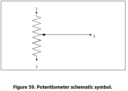
Potentiometer

The schematic symbol for the potentiometer is shown in Figure 59. The potentiometer  is  considered a three terminal device. As illustrated, terminals 1 and 2 have the entire value of the potentiometer resistance between them. Terminal 3 is the wiper or moving contact. Through this wiper, the resistance between terminals 1 and 3 or terminals 2 and 3 can be varied. While the rheostat is used to vary the current in a circuit, the potentiometer is used to vary the voltage in a circuit. A typical use for this component can be found in the volume controls on an audio panel and input devices for flight data recorders, among many other applications.

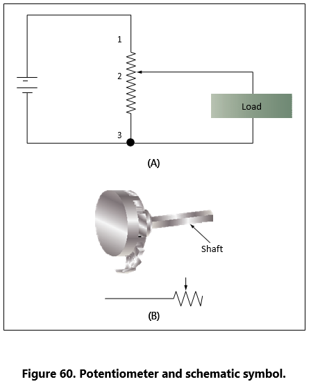
In Figure 60A, a potentiometer is used to obtain a variable voltage from a fixed voltage source to apply to an electrical load. The voltage applied to the load is the voltage between points 2 and 3. When the slider arm is moved to point 1, the entire voltage is applied to the electrical device (load); when the arm is moved to point 3, the voltage applied to the load is zero. The potentiometer makes possible the application of any voltage between zero and full voltage to the load.

The current flowing through the circuit of Figure 60 leaves the negative terminal electron flow of the battery and divides, one part flowing through the lower portion of the potentiometer (points 3 to 2) and the other part through the load. Both parts combine at point 2 and flow through the upper portion of the potentiometer (points 2 to 1) back to the positive terminal of the bat-tery. In View B of Figure 60, a potentiometer and its schematic symbol are shown.

In choosing a potentiometer resistance, the amount of current drawn by the load should be considered as well as the current flow through the potentiometer at all set- tings of the slider arm. The energy of the current through the potentiometer is dissipated in the form of heat.

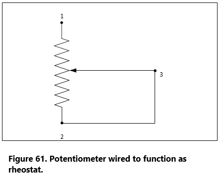
It is important to keep this wasted current as small as possible by making the resistance of the potentiometer as large as practicable. In most cases, the resistance of the potentiometer can be several times the resistance of the load. Figure 61 shows how a potentiometer can be wired to function as a rheostat.

Linear Potentiometers

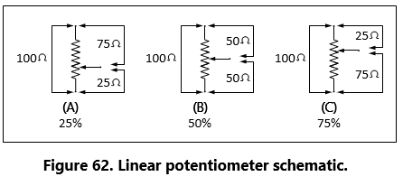
In a linear potentiometer, the resistance between both terminal and the wiper varies linearly with the position of the wiper. To illustrate, one quarter of a turn on the potentiometer will result in one quarter of the total resistance. The same relationship exists when one-half or three-quarters of potentiometer movement. Figure 62 schematically depicts this.

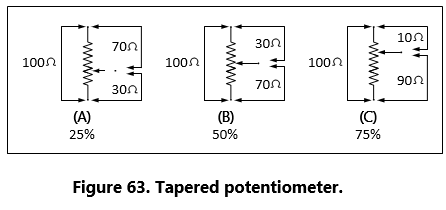
Tapered Potentiometers

Resistance varies in a nonlinear manner in the case of the tapered potentiometer. Figure 63 illustrates this. Keep in mind that one-half of full potentiometer travel doesn’t necessarily correspond to one-half the total resistance of the potentiometer.

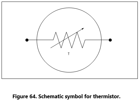
Thermistors

Figure 64 shows the schematic symbol for the thermistor. The thermistor is a type of a variable resis- tor, which is temperature sensitive. This component has what is known as a negative temperature coefficient, which means that as the sensed temperature increases, the resistance of the thermistor decreases.

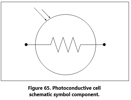
Photoconductive Cells

The photoconductive cell is similar to the thermis- tor. Like the thermistor, it has a negative temperature coefficient. Unlike the thermistor, the resistance is controlled by light intensity. This kind of component can be found in radio control heads where the intensity of the ambient light is sensed through the photoconductive cell resulting in the backlighting of the control heads to adjust to the cockpit lighting conditions. Figure 65 shows the schematic symbol component.

Chapter: 7 Circuit Protection Devices

Perhaps the most serious trouble in a circuit is a direct short. The term, “direct short,” describes a situation in which some point in the circuit, where full system voltage is present, comes in direct contact with the ground or return side of the circuit. This establishes a path for current flow that contains no resistance other than that present in the wires carrying the current, and these wires have very little resistance.

Most wires used in electrical circuits are small gauge, and their current carrying capacity is quite limited. The size of the wires used in any given circuit is determined by the amount of current the wires are expected to carry under normal operating conditions. Any current flow in excess of normal, such as the case of a direct short, would cause a rapid generation of heat. If the excessive current flow caused by the short is left unchecked, the heat in the wire will continue causing perhaps a portion of the wire to melt and at the very least, open the circuit.

To protect electrical systems from damage and failure caused by excessive current, several kinds of protective devices are installed in the systems. Fuses, circuit breakers, thermal protectors, and arc fault circuit breakers are used for this purpose.

Circuit protective devices, as the name implies, all have a common purpose — to protect the units and the wires in the circuit. Some are designed primarily to protect the wiring and to open the circuit in such   a way as to stop the current flow when the current becomes greater than the wires can safely carry. Other devices are designed to protect a unit in the circuit by stopping the current flow to it when the unit becomes excessively warm.

Fuse

Figure 66 shows the schematic symbol for the fuse. Fuses are used to protect the circuit from over current conditions. The fuse is installed in the circuit so that all the current in the circuit passes through it. In most fuses, the strip of metal is made of an alloy of tin and bismuth, which will melt and open the circuit when the current exceeds the rated capacity of the fuse. For example, if a 5-amp fuse is placed into a circuit, the fuse will allow currents up to 5 amps to pass. Because the fuse is intended to protect the circuit, it is quite important that its capacity match the needs of the circuit in which it is used.

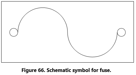
When replacing a fuse, consult the applicable manufacturer’s instructions to be sure a fuse of the correct type and capacity is installed. Fuses are installed in two types of fuse holders. “Plug-in holders” or in- line holders are used for small and low capacity fuses. “Clip” type holders are used for heavy high capacity fuses and current limiters.

Current Limiter

The current limiter is very much like the fuse. However, the current limiter link is usually made of copper and will stand a considerable overload for a short period of time. Like the fuse it will open up in an over current condition in heavy current circuits such as 30 amp or greater. These are used primarily to sectionalize an circuit or bus. Once the limiter is opened, it must    be replaced. The schematic symbol for the current limiter is the same as that for the fuse.

Circuit Breaker

The circuit breaker is commonly used in place of a fuse and is designed to break the circuit and stop the current flow when the current exceeds a predetermined value. Unlike the fuse, the circuit breaker can be reset; whereas the fuse or current limiter must be replaced. Figure 67 shows the schematic symbol for a circuit breaker.

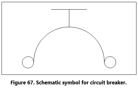
There are several types of circuit breakers in general use in electronic systems. One is a magnetic type. When excessive current flows in the circuit, it makes an electromagnet strong enough to move a small armature, which trips the breaker. Another type is the thermal overload switch or breaker. This consists of a bimetallic strip which, when it becomes overheated from exces- sive current, bends away from a catch on the switch lever and permits the switch to trip open.

Most circuit breakers must be reset by hand. If the overload condition still exists, the circuit breaker will trip again to prevent damage to the circuit. At this point, it is usually not advisable to continue resetting the circuit breaker, but to initiate troubleshooting to determine the cause. Repeated resetting of a circuit breaker can lead to circuit or component damage or worse, the possibility of a fire or explosion.

Arc Fault Circuit Breaker

In recent years, the arc fault circuit breaker has begun to provide an additional layer of protection beyond that of the thermal protection already provided by con- ventional circuit breakers. The arc fault circuit breaker monitors the circuit for an electrical arcing signature, which can indicate possible wiring faults and unsafe conditions. These conditions can lead to fires or loss of power to critical systems. The arc fault circuit breaker is only beginning to make an appearance in industry and is not widely used like the thermal type of circuit breaker.

Thermal Protectors

A thermal protector, or switch, is used to protect a motor. It is designed to open the circuit automatically whenever the temperature of the motor becomes exces- sively high. It has two positions— open and closed. The most common use for a thermal switch is to keep a motor from overheating. If a malfunction in the motor causes it to overheat, the thermal switch will break the circuit intermittently.

The thermal switch contains a bimetallic disk, or strip, which bends and breaks the circuit when it is heated. This occurs because one of the metals expands more than the other when they are subjected to the same temperature. When the strip or disk cools, the metals contract and the strip returns to its original position and closes the circuit.

Control Devices

Components in the electrical circuits are typically not all intended to operate continuously or automatically. Most of them are meant to operate at certain times, under certain conditions, to perform very definite func- tions. There must be some means of controlling their operation. Either a switch, or a relay, or both may be included in the circuit for this purpose.

Switches

Switches control the current flow in most elec-trical circuits. A switch is used to start, to stop, or to change the direction of the current flow in the circuit. The switch in each circuit must be able to carry the normal current of the circuit and must be insulated heavily enough for the voltage of the circuit.

An understanding of some basic definitions of the switch is necessary before any of the switch types are discussed. The number of poles, throws, and positions they have designates toggle switches, as well as some other type of switches.

Pole: the switch’s movable blade or contactor. The number of poles is equal to the number of circuits, or paths for current flow, that can be completed through the switch at any one time.

Throw: indicates the number of circuits, or paths for current, that it is possible to complete through the switch with each pole or contactor.

Positions: indicates the number of places at which the operating device (toggle, plunger, and so forth) will come to rest and at the same time open or close one or more circuits.

Toggle Switch

Single-Pole, Single-Throw (SPST)

The single-pole, single-throw switch allows a con- nection between two contacts. One of two conditions will exist. Either the circuit is open in one position or closed in the other position. The schematic symbol for this switch is shown in Figure 68.

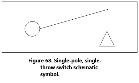
Single-Pole, Double-Throw (SPDT)

The single-pole, double-throw switch is shown in Figure 69. With this switch, contact between one con- tact can be made between one contact and the other.

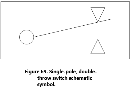
Double-Pole, Single-Throw (DPST)

The double-pole, single-throw switch connection can be made between one set of contacts and either of two other sets of contacts. The schematic symbol for this switch is shown in Figure 70.

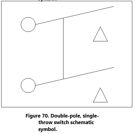
Double-Pole, Double-Throw (DPDT)

The schematic symbol for the double-pole, double- throw switch is shown in Figure 71. This type of switch makes a connection from one set of contacts to either of two other sets of contacts.

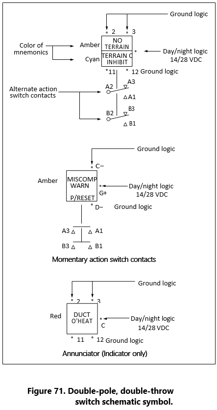
A toggle switch that is spring-loaded to the OFF position and must be held in the ON position to complete the circuit is a momentary contact two-position switch. One that will come to rest at either of two positions, opening the circuit in one position and closing it in another, is a two-position switch. A toggle switch that will come to rest at any one of three positions is a three-position switch.

A switch that stays open, except when it is held in the closed position, is a normally open switch (usually identified as NO). One that stays closed, except when it is held in the open position is a normally closed switch (NC). Both kinds are spring loaded to their normal position and will return to that position as soon as they are released.

Locking toggles require the operator to pull out on the switch toggle before moving it in to another position. Once in the new position, the switch toggle is release back into a lock, which then prevents the switch from inadvertently being moved.

Pushbutton Switches

Pushbutton switches have one stationary contact and one movable contact. The movable contact is attached to the pushbutton. The pushbutton is either an insulator itself or is insulated from the contact. This switch is spring loaded and designed for momentary contact.

Microswitches

A microswitch will open or close a circuit with a very small movement of the tripping device (1/16 inch or less). This is what gives the switch its name, since micro means small.

Microswitches are usually pushbutton switches. They are used primarily as limit switches to provide auto- matic control of landing gears, actuator motors, and the like. The diagram in Figure 72 shows a normally closed microswitch in cross-section and illustrates how these switches operate. When the operating plunger is pressed in, the spring and the movable contact are pushed, opening the contacts and the circuit.

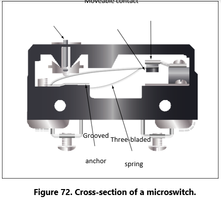
Rotary Selector Switches

A rotary selector switch takes the place of several switches. When the knob of the switch is rotated, the switch opens one circuit and closes another. Ignition switches and voltmeter selector switches are typical examples of this kind of switch. [Figure 73]

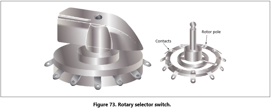
Lighted Pushbutton Switches

Another more common switch found in today’s electronics is the lighted pushbutton switch. This type of switch takes the form of a 5/8-inch to 1-inch cube with incandescent or LED lights to indicate the function of the switch. Switch designs come in a number of configurations; the two most common are the alternate action and momentary action and will usually have a two-pole or four-pole switch body. Other less com-mon switch actions are the alternate and momentary holding coil configurations. The less known holding or latching coil switch bodies are designed to have a magnetic coil inside the switch body that is energized through two contacts in the base of the switch. When the coil is energized and the switch is pressed, the switch contacts will  remain latched until power is removed from  the  coil. This type of design allows for some degree of remote control over the switch body. Figure 71 illustrates a schematic representation of this switch design.

The display optics of the lighted push button switch provide the crew with a clear message that is visible under a wide range of lighting conditions with very high luminance and wide viewing angles. While some displays are simply a transparent screen that is backlit by an incandescent light, the higher quality and more reliable switches are available in sunlight readable displays and night vision (NVIS) versions. Due to the sunlight environment of the cockpit, displays utilizing standard lighting techniques will “washout” when viewed in direct sunlight. Sunlight readable displays are designed to minimize this effect.

Lighted pushbutton switches can also be used in appli- cations where a switch is not required and the optics are only for indications. This type of an indicator is commonly called an annunciator.

DIP Switches

The acronym “DIP”switch is defined as DualIn-Line Parallel switch in reference to the physical layout. DIP switches are commonly found in card cages, and line replaceable units (LRU) are used in most cases to adjust gains, control configurations, and so forth. Each one of the switches is generally an SPST slide or rocker switch. The technician may find this switch in packages ranging in size from DIP2 through DIP32. Some of the more common sizes are DIP4 and DIP8.

Switch Guards

Switch guards are covers that protect a switch from unintended operation. Prior to the operation of the switch, the guard is usually lifted. Switch guards are commonly found on systems such as fire suppression and override logics for various systems.

Relays

A relay is simply an electromechanical switch where a small amount of current can control a large amount of current. Figure 74 illustrates the basic relay in both schematic and pictorial format. When a voltage is applied to the coil of the relay, the electromagnet will be energized due to the current. When energized, an electromagnetic field will pull the common (C)or arm of the relay down. When the arm or common is pulled down, the circuit between the arm and the normally closed (NC) contacts is opened and the circuit between the arm and the normally open (NO) contacts are closed. When the energizing voltage is removed, the spring will return the arm contacts back to the normally closed (NC) contacts. The relay usually has two connections for the coil. The (+) side is designated as X1 and the ground-side of the coil is designated as X2.

Chapter: 8 Series DC Circuits

Introduction

The series circuit is the most basic electrical circuit and provides a good introduction to basic circuit analysis. The series circuit represents the first building block for all of the circuits to be studied and analyzed. Figure 75 shows this simple circuit with nothing more than a voltage source or battery, a conductor, and a resistor. This is classified as a series circuit because the components are connected end-to-end, so that the same current flows through each component equally. There is only one path for the current to take and the battery and resistor are in series with each other. Next is to make a few additions to the simple circuit in Figure 75.

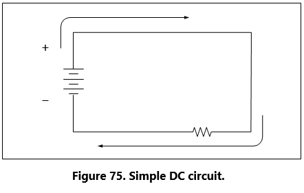
Figure 76 shows an additional resistor and a little more detail regarding the values. With these values, we can now begin to learn more about the nature of the circuit. In this configuration, there is a 12-volt DC source in series with two resistors, R1 = 10 Ω and    R2 = 30 Ω. For resistors in a series configuration, the total resistance of the circuit is equal to the sum of   the individual resistors. The basic formula is:

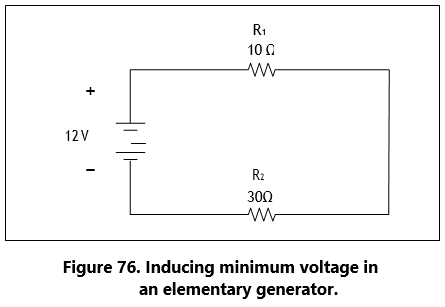
For Figure 76, this will be:

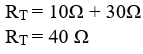
Now that the total resistance of the circuit is known, the current for the circuit can be determined. In a series circuit, the current cannot be different at different points within the circuit. The current through a series circuit will always be the same through each element and at any point. Therefore, the current in the simple circuit can now be determined using Ohm’s law:

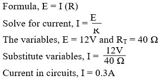
Ohm’s law describes a relationship between the vari- ables of voltage, current, and resistance that is linear and easy to illustrate with a few extra calculations.

First will be the act of changing the total resistance of the circuit while the other two remain constant.  In this example, the RT of the circuit in Figure 76 will be doubled. The effects on the total current in the circuit are:

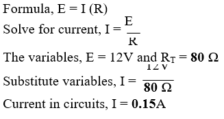
It can be seen quantitatively and intuitively that when the resistance of the circuit is doubled, the current is reduced by half the original value.

Next, reduce the RT of the circuit in Figure 76 to half of its original value. The effects on the total current are:

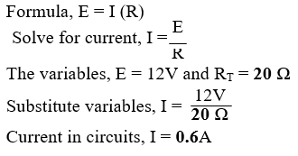
Voltage Drops and Further Application of Ohm’s Law

The example circuit in Figure 77 will be used to illustrate the idea of voltage drop. It is important to differentiate between voltage and voltage drop when discussing series circuits. Voltage drop refers to the loss in electrical pressure or emf caused by forcing electrons through a resistor. Because there are two resistors in the example, there will be separate voltage drops. Each drop is associated with each individual resistor. The amount of electrical pressure required to force a given number of electrons through a resistance is proportional to the size of the resistor.

In Figure 77, the values used to illustrate the idea of voltage drop are:

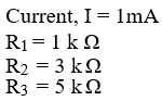
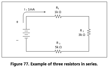
The voltage drop across each resistor will be calculated using Ohm’s law. The drop for each resistor is the product of each resistance and the total current in the circuit. Keep in mind that the same current flows through series resistor.

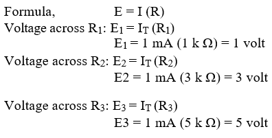
The source voltage can now be determined, which can then be used to confirm the calculations for each voltage drop. Using Ohm’s law:

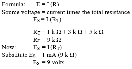
Simple checks to confirm the calculation and to illustrate the concept of the voltage drop add up the individual values of the voltage drops and compare them to the results of the above calculation.

1 volt + 3 volts + 5 volts = 9 volts.

Voltage Sources in Series

A voltage source is an energy source that provides   a constant voltage to a load. Two or more of these sources in series will equal the algebraic sum of all the sources connected in series. The significance of pointing out the algebraic sum is to indicate that the polarity of the sources must be considered when adding up the sources. The polarity will be indicated by a plus or minus sign depending on the source’s position in the circuit.

In Figure 78 all of the sources are in the same direction in terms of their polarity. All of the voltages have the same sign when added up. In the case of Figure 78, three cells of a value of 1.5 volts are in series with the polarity in the same direction. The addition is simple enough:

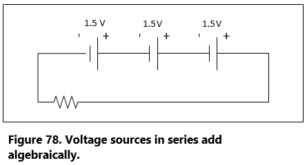
However, in Figure 79, one of the three sources has been turned around, and the polarity opposes the other two sources. Again the addition is simple:

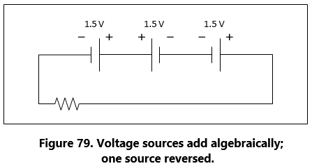
Kirchhoff’s Voltage Law

A law of basic importance to the analysis of an electrical circuit is Kirchhoff’s voltage law. This law simply states that the algebraic sum of all voltages around a closed path or loop is zero. Another way of saying it: The sum of all the voltage drops equals the total source voltage. A simplified formula showing this law is shown below:

With three resistors in the circuit:

Notice that the sign of the source is opposite that of the individual voltage drops. Therefore, the algebraic sum equals zero. Written another way:

The source voltage equals the sum of the voltage drops.

The polarity of the voltage drop is determined by the direction of the current flow. When going around the circuit, notice that the polarity of the resistor is opposite that of the source voltage. The positive on the resistor is facing the positive on the source and the negative towards the negative.

Figure 80 illustrates the very basic idea of Kirchhoff’s voltage law. There are two resistors in this example. One has a drop of 14 volts and the other has a drop of 10 volts. The source voltage must equal the sum of the voltage drops around the circuit. By inspection it is easy to determine the source voltage as 24 volts.

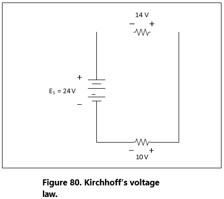
Figure 81 shows a series circuit with three voltage drops and one voltage source rated at 50 volts. Two of the voltage drops are known. However, the third is not known. Using Kirchhoff’s voltage law, the third voltage drop can be determined.

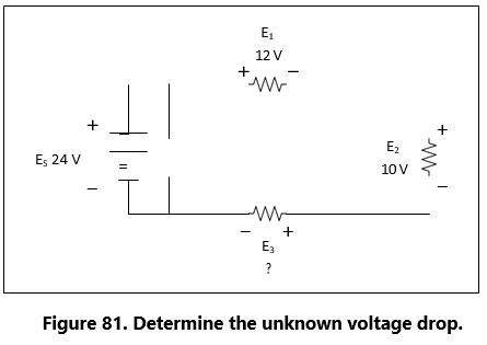
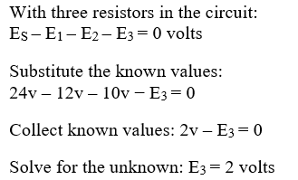
Determine the value of E4 in Figure 82. For this example, I = 200 mA.

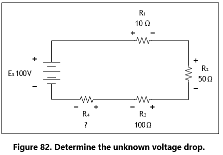
First, the voltage drop across each of the individual resistors must be determined.

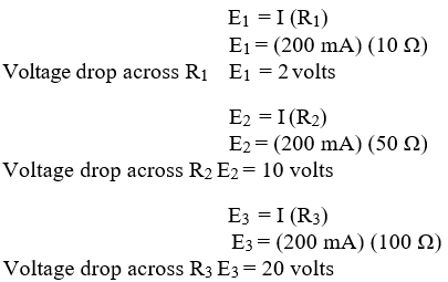
Kirchhoff’s voltage law is now employed to determine the voltage drop across E4.

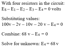
Using Ohm’s law and substituting in E4, the value for R4 can now be determined.

Voltage Dividers

Voltage dividers are devices that make it possible to obtain more than one voltage from a single power source. A voltage divider usually consists of a resistor, or resistors connected in series, with fixed or movable contacts and two fixed terminal contacts. As current flows through the resistor, different voltages can be obtained between the contacts.

Series circuits are used for voltage dividers. The volt- age divider rule allows the technician to calculate the voltage across one or a combination of series resistors without having to first calculate the current in the circuit. Because the current flows through each resistor, the voltage drops are proportional to the ohmic values of the constituent resistors.

A typical voltage divider is shown in Figure 83.

To understand how a voltage divider works, examine Figure 84 carefully and observe the following:

Each load draws a given amount of current: I1, I2, I3. In addition to the load currents, some bleeder current (IB) flows. The current (IT) is drawn from the power source and is equal to the sum of all currents.

The voltage at each point is measured with respect to a common point. Note that the common point is the point at which the total current (IT) divides into separate currents (I1, I2, I3).

Each part of the voltage divider has a different current flowing in it. The current distribution is as follows:

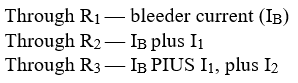
The voltage across each resistor of the voltage divider is:

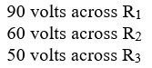
The voltage divider circuit discussed up to this point has had one side of the power supply (battery) at ground potential. In Figure 85 the common reference point (ground symbol) has been moved to a different point on the voltage divider. The voltage drop across R1 is 20 volts; however, since tap A is connected to  a point in the circuit that is at the same potential as the negative side of the battery, the voltage between tap A and the reference point is a negative (−) 20 volts. Since resistors R2 and R3 are connected to the positive side of the battery, the voltages between the reference point and tap B or C are positive.

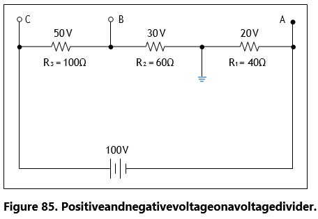
The following rules provide a simple method of deter- mining negative and positive voltages: (1) If current enters a resistance flowing away from the reference point, the voltage drop across that resistance is positive in respect to the reference point; (2) if current flows out of a resistance toward the reference point, the voltage drop across that resistance is negative in respect to the reference point. It is the location of the reference point that determines whether a voltage is negative or positive.

Tracing the current flow provides a means for determining the voltage polarity. Figure 86 shows the same circuit with the polarities of the voltage drops and the direction of current flow indicated.

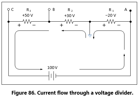
The current flows from the negative side of the battery to R1. Tap A is at the same potential as the negative terminal of the battery since the slight voltage drop caused by the resistance of the conductor is disregarded; however, 20 volts of the source voltage are required to force the current through R1 and this 20-volt drop has the polarity indicated. Stated another way, there are only 80 volts of electrical pressure left in the circuit on the ground side of R1.

When the current reaches tap B, 30 more volts have been used to move the electrons through R2, and in a similar manner the remaining 50 volts are used for R3. But the voltages across R2 and R3 are positive voltages, since they are above ground potential.

Figure 87 shows the voltage divider used previously. The voltage drops across the resistances are the same; however, the reference point (ground) has been changed. The voltage between ground and tap A is now a negative 100 volts, or the applied voltage.

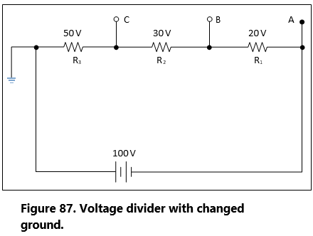
The voltage between ground and tap B is a negative 80 volts, and the voltage between ground and tap C is a negative 50 volts.

Determining the Voltage Divider Formula

Figure 88 shows the example network of four resistors and a voltage source. With a few simple calculations, a formula for determining the voltage divisions in a series circuit can be determined.

The voltage drop across any particular resistor shall be called EX, where the subscript x is the value of a particular resistor (1, 2, 3, or 4). Using Ohm’s law, the voltage drop across any resistor can be determined.

As seen earlier in the text, the current is equal to the source voltage divided by the total resistance of the series circuit.

The current equation can now be substituted into the equation for Ohm’s law.

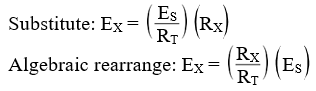
This equation is the general voltage divider formula. The explanation of this formula is that the voltage drop across any resistor or combination of resistors in a series circuit is equal to the ratio of the resistance value to the total resistance, divided by the value    of the source voltage. Figure 89 illustrates this with a network of three resistors and one voltage source.

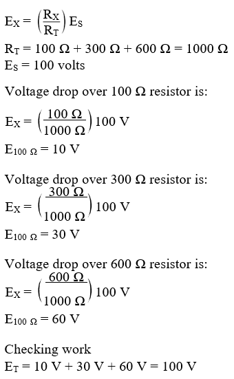
Chapter: 9 Parallel DC Circuits

Overview

A circuit in which two of more electrical resistances or loads are connected across the same voltage source is called a parallel circuit. The primary difference between the series circuit and the parallel circuit is that more than one path is provided for the current in the parallel circuit. Each of these parallel paths is called a branch. The minimum requirements for a parallel circuit are the following:

• A power source.
• Conductors.
• A resistance or load for each current path.
• Two or more paths for current flow.

Figure 90 depicts the most basic parallel circuit. Current flowing out of the source divides at point A in the diagram and goes through R1 and R2. As more branches are added to the circuit, more paths for the source current are provided.

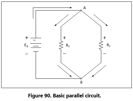
Voltage Drops

The first point to understand is that the voltage across any branch is equal to the voltage across all of the other branches.

Total Parallel Resistance

The voltage across any branch is equal to the voltage across all of the other branches.

The parallel circuit consists of two or more resistors connected in such a way as to allow current flow to pass through all of the resistors at once. This eliminates the need for current to pass one resistor before passing through the next. When resistors are connected in parallel, the total resistance of the circuit decreases. The total resistance of a parallel combination is always less than the value of the smallest resistor in the circuit. In the series circuit, the current has to pass through the resistors one at a time. This gave a resistance to the current equal the sum of all the resistors. In the parallel circuit, the current has several resistors that it can pass through, actually reducing the total resistance of the circuit in relation to any one resistor value.

The amount of current passing through each resistor will vary according to its individual resistance. The total current of the circuit will then be the sum of the current in all branches. It can be determined by inspection that the total current will be greater than that of any given branch. Using Ohm’s law to calculate the resistance based on the applied voltage and the total current, it can be determined that the total resistance is less than any individual branch.

An example of this is if there was a circuit with a 100 Ω resistor and a 5 Ω resistor; while the exact value must be calculated, it still can be said that the combined resistance between the two will be less than the 5 Ω.

Resistors in Parallel

The formula for the total parallel resistance is as follows:

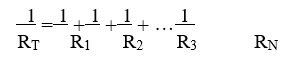
If the reciprocal of both sides is taken, then the general formula for the total parallel resistance is:

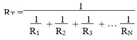
Two Resistors in Parallel

Typically, it is more convenient to consider only two resistors at a time because this setup occurs in common practice. Any number of resistors in a circuit can be broken down into pairs. Therefore, the most common method is to use the formula for two resistors  in parallel.

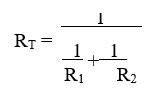
Combining the terms in the denominator and rewriting

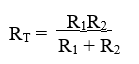
Put in words, this states that the total resistance for two resistors in parallel is equal to the product of both resistors divided by the sum of the two resistors. In the formula below, calculate the total resistance.

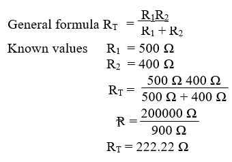
Current Source

A current source is an energy source that provides a constant value of current to a load even when the load changes in resistive value. The general rule to remember is that the total current produced by current sources in parallel is equal to the algebraic sum of the individual sources.

Kirchhoff’s Current Law

Kirchhoff’s current law can be stated as: The sum of the currents into a junction or node is equal to the sum of the currents flowing out of that same junction or node. Aj unction can be defined as a point in the circuit where two or more circuit paths come together. In the case of the parallel circuit, it is the point in the circuit where the individual branches join.

General formula   IT = I1 + I2 + I3

Refer to Figure 91 for an illustration. Point A and point B represent two junctions or nodes in the circuit with three resistive branches in between. The voltage source provides a total current IT into node A. At this point, the current must divide, flowing out of node A into each of the branches according to the resistive value of each branch. Kirchhoff’s current law states that the current going in must equal that going out. Following the current through the three branches and back into node B, the total current IT entering node B and leaving node B is the same as that which entered node A. The current then continues back to the volt- age source.

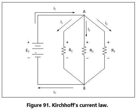
Figure 92 shows that the individual branch currents are:

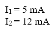
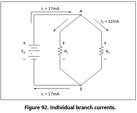
The total current flow into the node A equals the sum of the branch currents, which is:

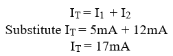
The total current entering node B is also the same.

Figure 93 illustrates how to determine an unknown current in one branch. Note that the total current into a junction of the three branches is known. Two of the branch currents are known. By rearranging the general formula, the current in branch two can be determined.

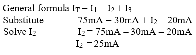
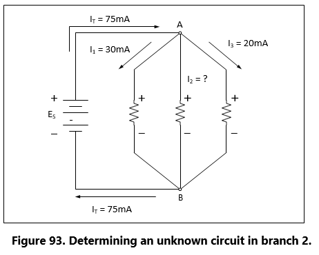
Current Dividers

It can now be easily seen that the parallel circuit is a current divider. As could be seen in Figure 90, there is a current through each of the two resistors. Because the same voltage is applied across both resistors in parallel, the branch currents are inversely proportional to the ohmic values of the resistors. Branches with higher resistance have less current than those with lower resistance. For example, if the resistive value of R2 is twice as high as that of R1, the current in R2 will be half of that of R1. All of this can be determined with Ohm’s law.

By Ohm’s law, the current through any one of the branches can be written as:

The voltage source appears across each of the parallel resistors and RX represents any one the resistors. The source voltage is equal to the total current times the total parallel resistance.

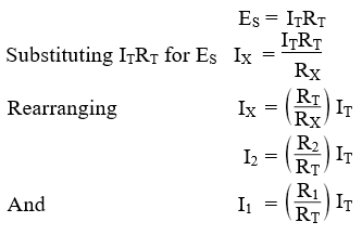
This formula is the general current divider formula. The current through any branch equals the total parallel resistance divided by the individual branch resistance, multiplied by the total current.

Series-Parallel DC Circuits

Overview

Most of the circuits that the technician will encounter will not be a simple series or parallel circuit. Circuits are usually a combination of both, known as series-parallel circuits, which are groups consisting of resistors in parallel and in series. An example of this type of circuit can be seen in Figure 94. While the series- parallel circuit can initially appear to be complex, the same rules that have been used for  the  series and parallel circuits can be applied to these circuits.

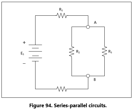
The voltage source will provide a current out to resistor R1, then to the group of resistors R2 and R3 and then to the next resistor R4 before returning to the voltage source. The first step in the simplification process is to isolate the group R2 and R3 and recognize that they are a parallel network that can be reduced to an equivalent resistor. Using the formula for parallel resistance,

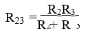
R2 and R3 can be reduced to R23. Figure 95 now shows an equivalent circuit with three series connected resistors. The total resistance of the circuit can now be simply determined by adding up the values of resistors R1, R23, and R4.

Determining the Total Resistance

A more quantitative example for determining total resistance and the current in each branch in a combination circuit is shown in the following example. Also refer to Figure 96.

The first step is to determine the current at junction A, leading into the parallel branch. To determine the IT, the total resistance RT of the entire circuit must be known. The total resistance of the circuit is given as:

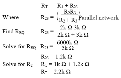
With the total resistance R_T now determined, the total IT can be determined. Using Ohm’s law:

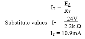
The current through the parallel branches of R2 and R3 can be determined using the current divider rule discussed earlier in the text. Recall that:

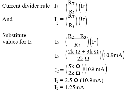
Now using Kirchhoff’s current law, the current in branch with R3 can be determined.

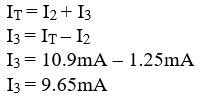
Chapter: 10 Alternating Current and Voltage

Alternating current has largely replaced direct current in commercial power systems for a number of reasons. It can be transmitted over long distances more readily and more economically than direct current, since AC voltages can be increased or decreased by means of transformers.

Because more and more units are being operated electrically in airplanes, the power requirements are such that a number of advantages can be realized by using AC. Space and weight can be saved, since AC devices, especially motors, are smaller and simpler than DC devices. In most AC motors no brushes are required, and commutation trouble at high altitude is eliminated. Circuit breakers will operate satisfactorily under load at high altitudes in an AC system, whereas arcing is so excessive on DC systems that circuit breakers must be replaced frequently. Finally, most airplanes using a 24- volt DC system have special equipment that requires a certain amount of 400 cycle AC current.

AC and DC Compared

“AC” stands for Alternating Current. Many of the prin- ciples, characteristics, and effects of AC are similar to those of direct current. Similarly, there are a number of differences, which will be explained. Direct current flows constantly in only one direction with a constant polarity. It changes magnitude only when the circuit is opened or closed, as shown in the DC waveform in Figure 97. Alternating current changes direction  at regular intervals, increases in value at a definite rate from zero to a maximum positive strength, and decreases back to zero; then it flows in the opposite direction, similarly increasing to a maximum nega- tive value, and again decreasing to zero. DC and AC waveforms are compared in Figure 97.

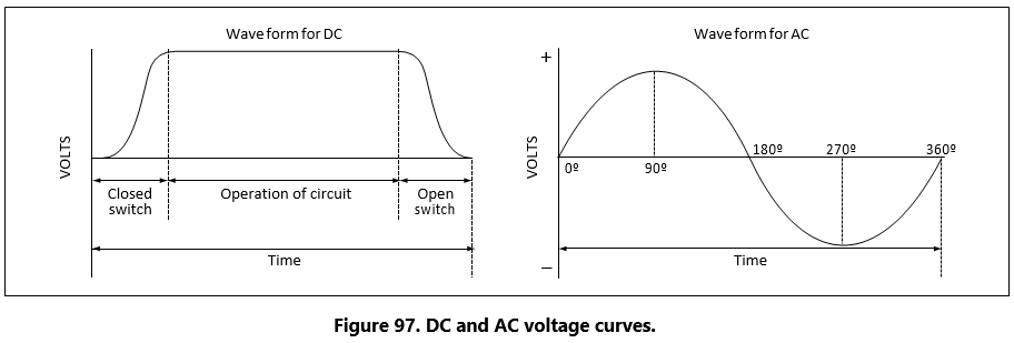
Since alternating current constantly changes direction and intensity, the following two effects (to be discussed later) take place in AC circuits that do not occur in DC circuits:

1. Inductive reactance.
2. Capacitive reactance.

Generator Principles

After the discovery that an electric current flowing through a conductor creates a magnetic field around the conductor, there was considerable scientific speculation about whether a magnetic field could create a current flow in a conductor. In 1831, it was demonstrated this could be accomplished.

To show how an electric current can be created by a magnetic field, a demonstration similar to that illus- trated in Figure 98 can be used. Several turns of a conductor are wrapped around a cylindrical form, and the ends of the conductor are connected together to form a complete circuit, which includes a galva- nometer. If a simple bar magnet is plunged into the cylinder, the galvanometer can be observed to deflect in one direction from its zero (center) position (Figure 98A).

When the magnet is at rest inside the cylinder, the galvanometer shows a reading of zero, indicating that no current is flowing (Figure 98B).

In Figure 98C, the galvanometer indicates a  cur- rent flow in the opposite direction when the magnet is pulled from the cylinder.

The same results may be obtained by holding the mag- net stationary and moving the cylinder over the magnet, indicating that a current flows when there is relative motion between the wire coil and the magnetic field. These results obey a law first stated by the German scientist, Heinrich Lenz. Lenz’s law states:

The induced current caused by the relative motion of a conductor and a magnetic field always flows in such a direction that its magnetic field opposes the motion.

Whena conductor is moved through a magnetic field, an electromotive force (emf) is induced in the con- ductor. [Figure 99] The direction (polarity) of the induced emf is determined by the magnetic lines of force and the direction the conductor is moved through the magnetic field. The generator left-hand rule (not to be confused with the left-hand rules used with a coil) can be used to determine the direction of the induced emf. [Figure 100] The left-hand rule is summed up as follows:

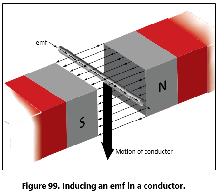
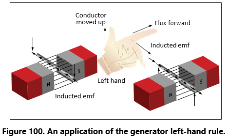
The first finger of the left hand is pointed in the direc- tion of the magnetic lines of force (north to south), the thumb is pointed in the direction of movement of the conductor through the magnetic field, and the second finger points in the direction of the induced emf.

When a loop conductor is rotated in a magnetic field, a voltage is induced in each side of the loop. [Figure 101] The two sides cut the magnetic field in opposite directions, and although the current flow is continuous, it moves in opposite directions with respect to the two sides of the loop. If sides A and B and the loop are rotated half a turn and the sides of the conductor have exchanged positions, the induced emf in each wire reverses its direction, since the wire formerly cutting the lines of force in an upward direction is now moving downward.

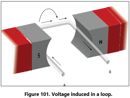
The value of an induced emf depends on three factors:

1. The number of wires moving through the magnetic field.
2. The strength of the magnetic field.
3. The speed of rotation.

Generators of Alternating Current

Generators used to produce an alternating current are called AC generators or alternators.

The simple generator constitutes one method of generating an alternating voltage. [Figure 102] It consists of a rotating loop, marked A and B, placed between two magnetic poles, N and S. The ends of the loop are connected to two metal slip rings (collector rings), C1 and C2. Current is taken  from the collector rings by brushes. If the loop is considered as separate wires A and B, and the left- hand rule for generators is applied, then it can be observed that as wire A moves up across the field, a voltage is induced which causes the cur-rent to flow inward. As wire B moves down across the field, a voltage is induced which causes the current to flow outward. When the wires are formed into a loop, the voltages induced in the two sides of the loop are combined. Therefore, for explanatory purposes, the action of either conductor, A or B, while rotating in the magnetic field is similar to the action of the loop.

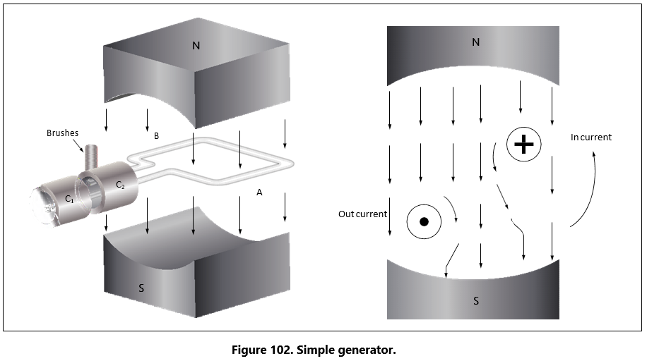
Figure 103 illustrates the generation of alternating current with a simple loop conductor rotating in a magnetic field. As it is rotated in a counterclockwise direction, varying values of voltages are induced in it.

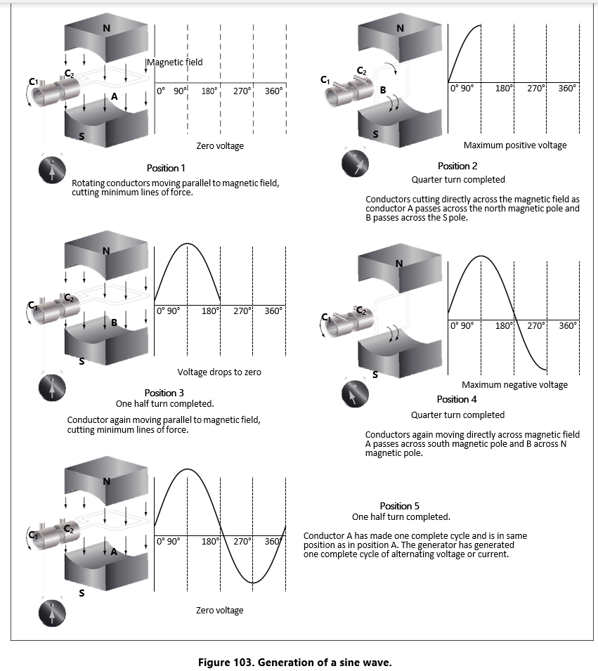
Position 1

The conductor A moves parallel to the lines of force. Since it cuts no lines of force, the induced voltage is zero. As the conductor advances from position 1 to position 2, the voltage induced gradually increases.

Position 2

The conductor is now moving perpendicular to the flux and cuts a maximum number of lines of force; therefore, a maximum voltage is induced. As the con- ductor moves beyond position 2, it cuts a decreasing amount of flux at each instant, and the induced voltage decreases.

Position 3

At this point, the conductor has made one-half of a revolution and again moves parallel to the lines of force, and no voltage is induced in the conductor. As the A conductor passes position 3, the direction of induced voltage now reverses since the A conductor is moving downward, cutting flux in the opposite direction. As the A conductor moves across the south pole, the induced voltage gradually increases in a negative direction, until it reaches position 4.

Position 4

Like position 2, the conductor is again moving perpendicular to the flux and generates a maximum negative voltage. From position 4 to 5, the induced voltage gradually decreases until the voltage is zero, and the conductor and wave are ready to start another cycle.

Position 5

The curve shown at position 5 is called a sine wave. It represents the polarity and the magnitude of the instantaneous values of the voltages generated. The horizontal base line is divided into degrees, or time, and the vertical distance above or below the base line represents the value of voltage at each particular point in the rotation of the loop.

Cycle and Frequency

Cycle Defined

A cycle is a repetition of a pattern. Whenever a voltage or current passes through a series of changes, returns to the starting point, and then again starts the same series of changes, the series is called a cycle. The cycle is represented by the symbol of a wavy line in a circle . In the cycle of voltage shown in Figure 104. the voltage increases from zero to a maximum positive value, decreases to zero; then increases to a maximum negative value, and again decreases to zero. At this point, it is ready to go through the same series of changes. There are two alternations in a complete cycle: the positive alternation and the negative.  Each is half a cycle.

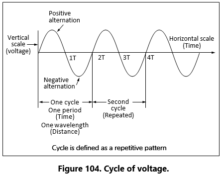
Frequency Defined

The frequency is the number of cycles of alternating current per second (1 second). The standard unit of frequency measurement is the hertz (Hz). [Figure 105]

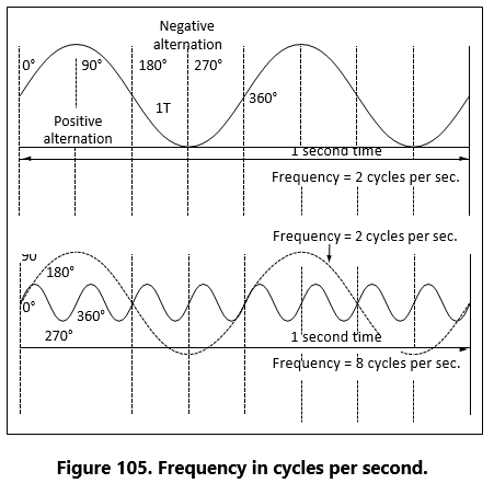
In a generator, the voltage and current pass through a complete cycle of values each time a coil or conductor passes under a north and south pole of the magnet. The number of cycles for each revolution of the coil or conductor is equal to the number of pairs of poles. The frequency, then, is equal to the number of cycles in one revolution multiplied by the number of revolutions per second. Expressed in equation form,

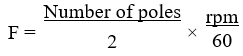
where ^P⁄2 is the number of pairs of poles, and rpm/60 the number of revolutions per second. If in a 2 pole generator, the conductor is turning at 3,600 rpm, the revolutions per second are

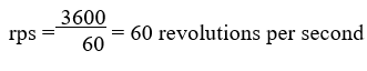
Since there are 2 poles, ^P⁄2  is 1, and the frequency   is 60 cycles per second (cps). In a 4 pole generator with an armature speed of 1,800 rpm, substitute in the equation,

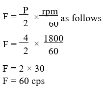
Period Defined

The time required for a sine wave to complete one full cycle is called a period. [Figure 104] The period of a sine wave is inversely proportional to the frequency. That is to say that the higher the frequency, the shorter the period will be. The mathematical relationship between frequency and period is given as:

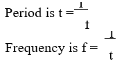
Wavelength Defined

The distance that a waveform travels during a period is commonly referred to as a wavelength and is indicated by the Greek letter lambda (λ). The measurement of wavelength is taken from one point on the waveform to a corresponding point on the next waveform. [Figure 104]

Phase Relationships

In addition to frequency and cycle characteristics, alternating voltage and current also have a relationship called “phase.” In a circuit that is fed (supplied) by one alternator, there must be a certain phase relationship between voltage and current if the circuit is to function efficiently. In a system fed by two or more alternators, not only must there be a certain phase relationship between voltage and current of one alternator, but there must be a phase relationship between the indi- vidual voltages and the individual currents. Also, two separate circuits can be compared by comparing the phase characteristics of one to the phase characteristics of the other.

In Phase Condition

Figure 106A, shows a voltage signal and a current signal superimposed on the same time axis. Notice that when the voltage increases in the positive alter- nation that the current also increases. When the voltage reaches it peak value, so does the current. Both waveforms then reverse and decrease back to a zero magnitude, then proceed in the same manner in the negative direction as they did in the positive direction. When two waves, such as these in Figure 106A, are exactly in step with each other, they are said to be in phase. To be in phase, the two waveforms must go through their maximum and minimum points at the same time and in the same direction.

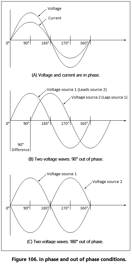
Out of Phase Condition

When two waveforms go through their maximum and minimum points at different times, a phase difference will exist between the two. In this case, the two wave-forms are said to be out of phase with each other. The terms lead and lag are often used to describe the phase difference between waveforms. The waveform that reaches its maximum or minimum value first is said to lead the other waveform. Figure 106B shows this relationship. Voltage source one starts to rise at the 0° position and voltage source two starts to rise at the 90° position. Because voltage source one begins its rise earlier in time (90°) in relation to the second voltage source, it is said to be leading the second source. On the other hand, the second source is said to be lagging the first source. When a waveform is said to be leading or lagging, the difference in degrees is usually stated. If the two waveforms differ by 360°, they are said to be in phase with each other. If there is a 180° difference between the two signals, then they are still out of phase even though they are both reaching their minimum and maximum values at the same time. [Figure 106]

Values of Alternating Current

There are three values of alternating current, which are instantaneous, peak, and effective (root mean square, RMS).

Instantaneous Value

An instantaneous value of voltage or current is the induced voltage or current flowing at any instant dur-ing a cycle. The sine wave represents a series of these values. The instantaneous value of the voltage varies from zero at 0° to maximum at 90°, back to zero at 180°, to maximum in the opposite direction at 270°, and to zero again at 360°. Any point on the sine wave is considered the instantaneous value of voltage.

Peak Value

The  peak  value  is  the  largest  instantaneous value. The largest single positive value occurs when the sine wave of voltage is at 90°, and the largest single negative value occurs when it is at 270°. Maximum value is 1.41 times the effective value. These are called peak values.

Effective Value

The effective value is also known as the RMS value or root mean square, which refers to the mathematical pro-cess by which the value is derived. Most AC voltmeters will display the effective or RMS value when used. The effective value is less than the maximum value, being equal to .707 times the maximum value. The effective value of a sine wave is actually a mea- sure of the heating effect of the sine wave. Figure 107 illustrates what happens when a resistor is connected across an AC voltage source. In illustra- tion A, a certain amount of heat is generated by the power in the resistor. Illustration B shows the same resistor now inserted into a DC voltage source. The value of the DC voltage source can now be adjusted so  that the resistor dissipates the same amount  of heat as it did when it was in  the AC  circuit. The RMS or effective value of a sine wave is equal to the DC voltage that produces the same amount of heat as the sinusoidal voltage.

The peak value of a sine wave can be converted to the corresponding RMS value using the following relationship.

Vrms = ( √ 0.5 ) × Vp

Vrms = 0.707 × Vp

This can be applied to either voltage or current.

Algebraically rearranging the formula and solving for Vp can also determine the peak voltage. The resulting formula is:

Vp = 1.414 × Vrms

Thus, the 110 volt value given for alternating current supplied to homes is only 0.707 of the maximum voltage of this supply. The maximum voltage is approximately 155 volts.

In the study of alternating current, any values given for current or voltage are assumed to be effective values unless otherwise specified, and in practice, only the effective values of voltage and current are used. Similarly, alternating current voltmeters and ammeters measure the effective value.

Chapter: 11 Capacitance

Another important property in AC circuits, besides resistance and inductance, is capacitance. While induc- tance is represented in a circuit by a coil, capacitance is represented by a capacitor. In its most basic form the capacitor is constructed of two parallel plates separated by a nonconductor, called a dielectric. In an electrical circuit, a capacitor serves as a reservoir or storehouse for electricity.

Capacitors in Direct Current

When a capacitor is connected across a source of direct current, such as a storage battery in the circuit shown in Figure 108A, and the switch is then closed, the plate marked B becomes positively charged, and the A plate negatively charged. Currentflows in the external circuit during the time the electrons are moving from B to A. The current flow in the circuit is at a maximum the instant the switch is closed, but continually decreases thereafter until it reaches zero. The current becomes zero as soon as the difference in voltage of A and B becomes the same as the voltage of the battery. If the switch is opened as shown in Figure 108B, the plates remain charged. Once the capacitor is shorted, it will discharge quickly as shown Figure 108C.

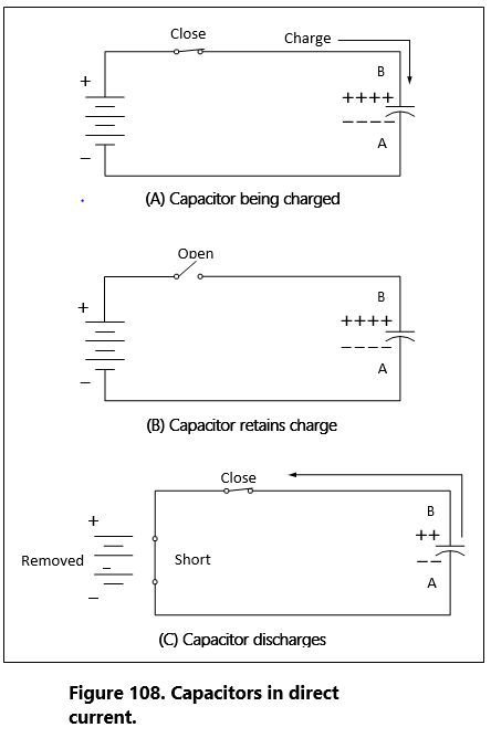
It should be clear that during the time the capacitor  is being charged or discharged, there is current in the circuit, even though the circuit is broken by the gap between the capacitor plates. Current is present only during the time of charge and discharge, and this period of time is usually short.

The RC Time Constant

The time required for a capacitor to attain a full charge is proportional to the capacitance and the resistance of the circuit. The resistance of the circuit introduces the element of time into the charging and discharging of a capacitor.

When a capacitior charges or discharges through a resistance, a certain amount of time is required for a full charge or discharge. The voltage across the capacitor will not change instantaneously. The rate of charging or discharging is determined by the time constant of the circuit. The time constant of a series RC (resis-tor/capacitor) circuit is a time interval that equals the product of the resistance in ohms and the capacitance in farad and is symbolized by the greek letter tau (τ).

τ=RC

The time in the formula is that required to charge to 63% of the voltage of the source. The time required to bring the charge to about 99% of the source voltage is approximately 5 τ. Figure 109 illustrates this relationship of a time constant characteristics of charging.

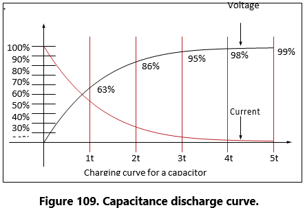
The measure of a capacitor’s ability to store charge is its capacitance. The symbol used for capacitance is the letter C.

As can be seen from the time constant illustration there can be no continuous movement of direct cur- rent through a capacitor. A good capacitor will block direct current and will pass the effects of pulsing DC or alternating current.

Units of Capacitance

Electrical charge, which is symbolized by the letter Q, is measured in units of coulombs. The coulomb is given by the letter C, as with capacitance. Unfortunately this can be confusing. One coulomb of charge is defined as a charge having 6.28 × 1018 electrons. The basic unit of capacitance is the farad and is given by the letter f. By definition, one farad is one coulomb of charge stored with one volt across the plates of the capacitor. The general formula for capacitance in terms of charge and voltage is:

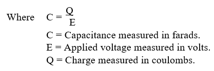
In practical terms, one farad is a large amount of capacitance. Typically, in electronics, much smaller units are used. The two more common smaller units are the microfarad (μF), which is 6 farad and the picofarad (pF), which is 12 farad.

Voltage Rating of a Capacitor

Capacitors have their limits as to how much voltage can be applied across the plates. The technician must be aware of the voltage rating, which specifies the maximum DC voltage that can be applied without the risk of damage to the device. This voltage rating is typically called the breakdown voltage, the working voltage, or simply the voltage rating. If the voltage applied across the plates is too great, the dielectric will break down and arcing will occur between the plates. The capacitor is then short circuited, and the possible flow of direct current through it can cause damage to other parts of the equipment.

A capacitor that can be safely charged to 500 volts DC cannot be safely subjected to AC or pulsating DC whose effective values are 500 volts. An alternating voltage of 500 volts (RMS) has a peak voltage of 707 volts, and a capacitor to which it is applied should have a working voltage of at least 750 volts. The capacitor should be selected so that its working voltage is at least 50 percent greater than the highest voltage to be applied.

The voltage rating of the capacitor is a factor in deter- mining the actual capacitance because capacitance decreases as the thickness of the dielectric increases. A high voltage capacitor that has a thick dielectric must have a larger plate area in order to have the same capacitance as a similar low voltage capacitor having a thin dielectric.

Factors Affecting Capacitance

1. The capacitance of parallel plates is directly proportional to their A larger plate area produces a larger capacitance and a smaller area produces less capacitance. If we double the area of the plates, there is room for twice as much charge. The charge that a capacitor can hold at a given potential difference is doubled, and since C = Q/ E, the capacitance is doubled.
2. The capacitance of parallel plates is inversely proportional to their spacing.
3. The dielectric material affects the capacitance of parallel The dielectric constant of a vacuum is defined as 1, and that of air is very close to
   1. These values are used as a reference, and all other materials have values specified in relation to air (vacuum).

The strength of some commonly used dielectric mate-rials is listed in Figure 110. The  voltage  rating also depends on frequency  because  the losses, and the resultant heating effect, increase as the frequency increases.

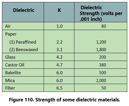
Types of Capacitors

Capacitors come in all shapes and sizes and are usu- ally marked with their value in farads. They may also be divided into two groups: fixed and variable. The fixed capacitors, which have approximately constant capacitance, may then be further divided according to the type of dielectric used. Some varieties are: paper, oil, mica, electrolytic and ceramic capacitors. Figure 111 shows the schematic symbols for a fixed and variable capacitor.

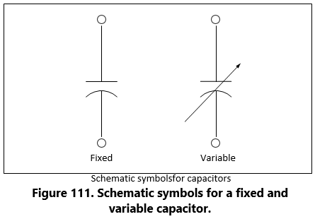
Fixed Capacitors

Mica Capacitors

The fixed mica capacitor is made of metal foil plates that are separated by sheets of mica, which form the dielectric. The whole assembly is covered in molded plastic, which keeps out moisture. Mica is an excellent dielectric and will withstand higher voltages than paper without allowing arcing between the plates. Common values of mica capacitors range from approximately 50 micromicrofarads, to about 0.02 microfarads.

Ceramic

The ceramic capacitor is constructed with materials, such as titanium acid barium for a dielectric. Internally these capacitors are not constructed as a coil, so they are well suited for use in high frequency applications. They are shaped like a disk, available in very small capacitance values  and very small sizes. This type  is fairly small, inexpensive, and reliable. Both the ceramic and the electrolytic are the most widely avail- able and used capacitor.

Electrolytic

Two kinds of electrolytic capacitors are in use: (1) wet electrolytic and (2) dry electrolytic.

The wet electrolytic capacitor is designed of two metal plates separated by an electrolyte with an electrolyte dielectric, which is basically conductive salt in solvent. For capacitances greater than a few microfarads, the plate areas of paper or mica capacitors must become very large; thus, electrolytic capacitors are usually used instead. These units provide large capacitance in small physical sizes. Their values range from 1 to about 1,500 microfarads. Unlike the other types, electrolytic capacitors are generally polarized, with the positive lead marked with a “+” and the negative lead marked with a “−” and should only be subjected to direct volt- age or pulsating direct voltage only.

The electrolyte in contact with the negative terminal, either in paste or liquid form, comprises the negative electrode. The dielectric is an exceedingly thin film of oxide deposited on the positive electrode of the capacitor. The positive electrode, which is an aluminum sheet, is folded to achieve maximum area. The capacitor is subjected to a forming process during manufacture, in which current is passed through it. The flow of current results in the deposit of the thin coating of oxide on the aluminum plate.

The close spacing of the negative and positive electrodes gives rise to the comparatively high capacitance value, but allows greater possibility of voltage break- down and leakage of electrons from one electrode to the other.

The electrolyte of the dry electrolytic unit is a paste contained in a separator made of an absorbent mate- rial, such as gauze or paper. The separator not only holds the electrolyte in place but also prevents it from short circuiting the plates. Dry electrolytic capacitors are made in both cylindrical and rectangular block form and may be contained either within cardboard or metal covers. Since the electrolyte cannot spill, the dry capacitor may be mounted in any convenient position. Electrolytic capacitors are shown in Figure 112.

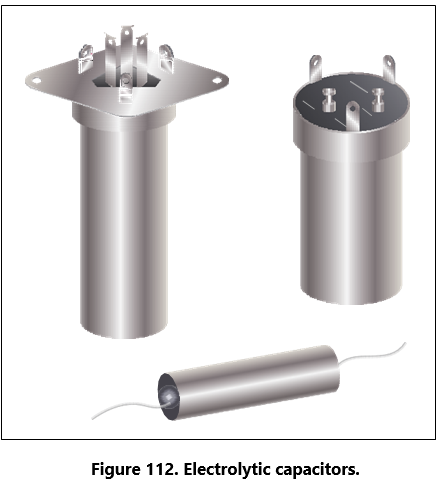
Tantalum

Similar to the electrolytic, these capacitors are constructed with a material called tantalum, which is used for the electrodes. They are superior to electrolytic capacitors, having better  temperature and frequency characteristics. When tantalum powder is baked in order to solidify it, a  crack  forms inside. This crack is used to store an electrical charge. Like electrolytic capacitors, the tantalum capacitors are also polarized and are indicated with the “+” and “−” symbols.

Polyester Film

In this capacitor, a thin polyester film is used as a dielectric. These components are inexpensive, temperature stable, and widely used. Tolerance is approximately 5 –10 percent. It can be quite large depending on capacity or rated voltage.

Oil Capacitors

In radio and radar transmitters, voltages high enough to cause arcing, or breakdown, of paper dielectrics are often used. Consequently, in these applications capacitors that use oil or oil impregnated paper for the dielectric material are preferred. Capacitors of this type are considerably more expensive than ordinary paper capacitors, and their use is generally restricted to radio and radar transmitting equipment. [Figure 113]

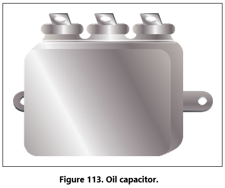
Variable Capacitors

Variable capacitors are mostly used in radio tuning circuits, and they are sometimes called “tuning capacitors.” They have very small capacitance values, typi- cally between 100pF and 500pF.

Trimmers

The trimmer is actually an adjustable or variable capacitor, which uses ceramic or plastic as a dielectric. Most of them are color coded to easily recognize their tunable size. The ceramic type has the value printed on them. Colors are: yellow (5pF), blue (7pF), white (10pF), green (30pF), and brown (60pf).

Varactors

A voltage-variable capacitor or varactor is also known as a variable capacitance diode or a varicap. This device utilizes the variation of the barrier width in a reversed-biased diode. Because the barrier width of a diode acts as a non-conductor, a diode forms a capacitor when reversed biased. Essentially the N-type material becomes one plate and the junctions are the dielectric. If the reversed-bias voltage is increased, then the barrier width widens, effectively separating the two capacitor plates and reducing the capacitance.

Capacitors in Series

When capacitors are placed in series, the effective plate separation is increased and the total capacitance is less than that of the smallest capacitor. Additionally, the series combination is capable of withstanding a higher total potential difference than any of the individual capacitors. Figure 114 is a simple  series  circuit.  The bottom plate of C1 and the top plate of C2 will  be charged by electrostatic induction. The capacitors charge as current is established through the circuit. Since this is a series circuit, the current must be the same at all points. Since the current is the rate of flow of charge, the amount of charge (Q) stored by each capacitor is equal to the total charge.

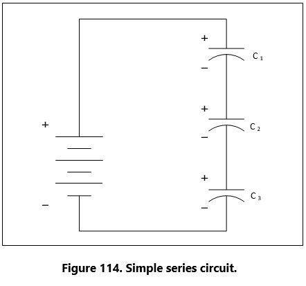
According to Kirchhoff’s voltage law, the sum of the voltages across the charged capacitors must equal the total voltage, ET. This is expressed as:

Equation E = Q/C can now be substituted into the voltage equation where we now get:

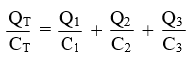
Since the charge on all capacitors is equal, the Q terms can be factored out, leaving us with the equation:

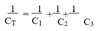
Consider the following example:

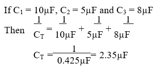
Capacitors in Parallel

When capacitors are connected in parallel, the effective plate area increases, and the total capacitance is the sum of the individual capacitances. Figure 115 shows a simplified parallel circuit. The total charging current from the source divides at the junction of the parallel branches. There is a separate charging current through each branch so that a different charge can be stored by each capacitor. Using Kirchhoff’s current law, the sum of all of the charging currents is then equal to the total current. The sum of the charges (Q) on the capacitors is equal to the total charge. The voltages (E) across all of the parallel branches are equal. With all of this in mind, a general equation for capacitors in parallel can be determined as:

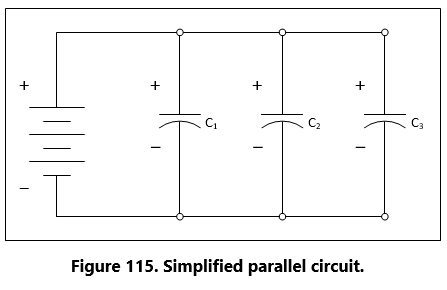
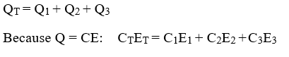
Voltages can be factored out because:

Leaving us with the equation for capacitors in parallel:

Consider the following example:

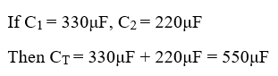
Capacitors in Alternating Current

If a source of alternating current is substituted for  the battery, the capacitor acts quite differently than  it does with direct current. When an alternating cur- rent is applied in the circuit, the charge on the plates constantly changes. [Figure 116] This means that electricity must flow first from Y clockwise around to X, then from X counterclockwise around to Y, then from Y clockwise around to X, and so on. Although no current flows through the insulator between the plates of the capacitor, it constantly flows in the remainder of the circuit between X and Y. In a circuit in which there is only capacitance, current leads the applied voltage as contrasted with a circuit in which there is inductance, where the current lags the voltage.

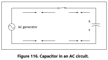
Capacitive Reactance Xc

The effectiveness of a capacitor in allowing an AC flow to pass depends upon the capacitance of the circuit and the applied frequency. To what degree a capacitor allows an AC flow to pass depends largely upon the capacitive value of the capacitor given in farads (f ). The greater the capacitance of the capacitor, the greater the number of electrons, measured in Coulombs, necessary to bring the capacitor to a fully charged state. Once the capacitor approaches or actually reaches a fully charged condition, the polarity of the capacitor will oppose the polarity of the applied voltage, essentially acting then as an open circuit. To further illustrate this characteristic and how it manifests itself in an AC circuit, consider the following. If a capacitor has a large capacitive value, meaning that it requires a relatively large number of electrons to bring it to a fully charged state, then a rather high frequency current can alternate through the capacitor without the capacitor ever reaching a full charge. In this case, if the frequency is high enough and the capacitance large enough that there is never enough time for the capacitor to ever reach a full charge, it  is possible that the capacitor may offer very little or no resistance to the current. However, the smaller the capacitance, the fewer electrons are required to bring it up to a full charge and it is more likely that the capacitor will build up enough of an opposing charge that it can present a great deal of resistance to the current if not to the point of behaving like an open circuit. In between these two extreme conditions lies a continuum of possibilities of current opposition depending on the combination of alpplied frequency and the selected capacitance. Current in an AC circuit can be controlled by changing the circuit capacitance in a similar manner that resistance can control the current. The actual AC reactance Xc, which just like resistance, is measured in ohms (Ω). Capacitive reactance Xc is determined by the following:

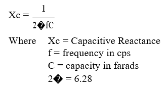
Sample Problem:

A series circuit is assumed in which the impressed voltage is 110 volts at 60 cps, and the capacitance of a condenser is 80 Mf. Find the capacitive reactance and the current flow.

Solution:

To find capacitive reactance, the equation Xc = 1/(2 p f C) is used. First, the capacitance, 80 Mf, is changed to farads by dividing 80 by 1,000,000, since 1 million microfarads is equal to 1 farad. This quotient equals 0.000080 farad. This is substituted in the equation and

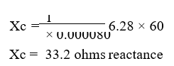
Once the reactance has been determined, ohm’s law can then be used in the same manner as it is used in DC circuits to determine the current.

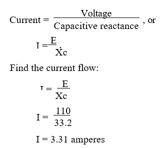
Capacitive Reactances in Series and in Parallel When capacitors are connected in series, the total reactance is equal to the sum of the individual reactances. Thus,

The total reactance of capacitors connected in parallel is found in the same way total resistance is computed in a parallel circuit: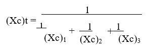

Phase of Current and Voltage in Reactive Circuits Unlike a purely resistive circuit, the capacitive and inductive reactance has a significant effect on the phase relationship between the applied AC voltage and  the corresponding current in the circuit.

In review, when current and voltage pass through zero and reach maximum value at the same time, the current and voltage are said to be in phase. [Figure 117A] If the current and voltage pass through zero and reach the maximum values at different times, the current and voltage are said to be out of phase. In a circuit containing only inductance, the current reaches a maximum value later than the voltage, lagging the voltage by 90°, or one-fourth cycle. [Figure 117B]

In a circuit containing only capacitance, the current reaches its maximum value ahead of the voltage and the current leads the voltage by 90°, or one-fourth cycle. [Figure 117C] The amount the current lags or leads the voltage in a circuit depends on the relative amounts of resistance, inductance, and capacitance in the circuit.

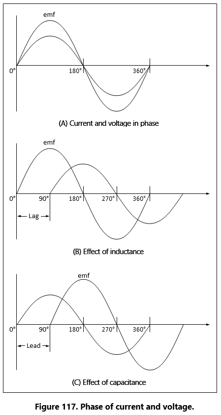
Chapter: 12 Inductance

Characteristics of Inductance

Michael Faraday discovered that by moving a magnet through a coil of wire, a voltage was induced across the coil. If a complete circuit was provided, then a cur- rent was also induced. The amount of induced voltage is directly proportional to the rate of change of the magnetic field with respect to the coil. The simplest of experiments can prove that when a bar magnet is moved through a coil of wire, a voltage is induced and can be measured on a voltmeter. This is commonly known as Faraday’s Law or the law of electromagnetic induction, which states:

The induced emf or electromagnetic force in a closed loop of wire is proportional to the rate of change of the magnetic flux through a coil of wire.

Conversely, current flowing through a coil of wire produces a magnetic field. When this wire is formed into a coil, it then becomes a basic inductor. The magnetic lines of force around each loop or turn in the coil effectively add to the lines of force around the adjoining loops. This forms a strong magnetic field within and around the coil. Figure 118A, illustrates  this idea of a coil of wire strengthening a magnetic field. The magnetic lines of force around adjacent loops are deflected into an outer path when the loops are brought close together. This happens because the magnetic lines of force between adjacent loops are in opposition with each other. The total magnetic field for the two loops is shown in Figure 118B. As more loops are added close together, the strength of the magnetic field will increase. Figure 118C illustrates the combined effects of many loops of a coil. The result is a strong electromagnet.

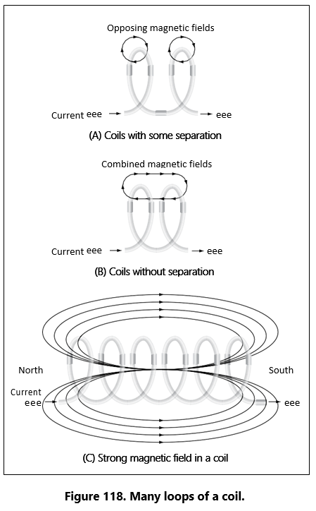
The primary aspect of the operation of a coil is its property to oppose any change in current through it. This property is called inductance. When current flows through any conductor, a magnetic field starts to expand from the center of the wire. As the lines of magnetic force grow outward through the conductor, they induce an emf in the conductor itself. The induced voltage is always in the direction opposite to the direction of the current flow. The effects of this countering emf are to oppose the immediate establishment of the maximum current. This effect is only a temporary condition. Once the current reaches a steady value in the conductor, the lines of magnetic force will no longer be expanding and the countering emf will no longer be present.

At the starting instant, the countering emf nearly equals the applied voltage, resulting in a small current flow. However, as the lines of force move outward, the num- ber of lines cutting the conductor per second becomes progressively smaller, resulting in a diminished counter emf. Eventually, the counter emf drops to zero and the only voltage in the circuit is the applied voltage and the current is at its maximum value.

The RL Time Constant

Because the inductors basic action is to oppose a change in its current, it then follows that the current cannot change instantaneously in the inductor. A certain time is required for the current to make a change from one value to another. The rate at which the current changes is determined by a time constant represented by the greek letter tau (τ). The time constant for the RL circuit is:

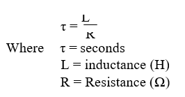
In a series RL circuit, the current will increase to 63% of its full value in 1 time constant after the circuit is closed. This build up of course is similar to the build up of voltage in a capacitor when charging an RC circuit. Both follow an exponential curve and reach 99% value after the 5th time constant. Figure 119 illustrates this characteristic.

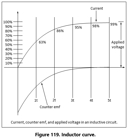
Physical Parameters

Some of the physical factors that affect inductance are:

1. The number of turns: Doubling the number of turns in a coil will produce a field twice as strong, if the same current is As a general rule, the inductance varies as the square of the number of turns.
2. The cross-sectional area of the coil: The inductance of a coil increases directly as the cross-sectional area of the core Doubling the radius of a coil increases the inductance by a factor of four.
3. The length of a coil: Doubling the length of a coil, while keeping the same number of turns, halves the value of inductance.
4. The core material around which the coil is formed: Coils are wound on either magnetic or nonmagnetic Some nonmagnetic materials include air, copper, plastic, and glass. Magnetic materials include nickel, iron, steel, or cobalt, which have a permeability that provides a better path for the magnetic lines of force and permit a stronger magnetic field.

Self-Inductance

The characteristic of self-inductance was summarized by German physicist Heinrich Lenz in 1833 and gives the direction of the induced electromotive force (emf) resulting from electromagnetic induction. This is com- monly known as Lenz’s Law, which states:

The emf induced in an electric circuit always acts in such a direction that the current it drives around a closed circuit produces a magnetic field which opposes the change in magnetic flux.

Self inductance is the generation of a voltage in an electric circuit by a changing current in the same circuit. Even a straight piece of wire will have some degree of inductance because current in a conductor produces a magnetic field. When the current in a conductor changes direction, there will be a corresponding change in the polarity of the magnetic field around the conductor. Therefore, a changing current produces a changing magnetic field around the wire. To further intensify the magnetic field, the wire can be rolled into a coil, which is called an inductor. The changing magnetic field around the inductor induces a voltage across the coil. This induced electromotive force is called self-inductance and tends to oppose any change in current within the circuit. This property is usually called inductance and symbolized with the letter L.

Types of Inductors

Inductors used in radio can range from a straight wire at UHF to large chokes and transformers used for filter- ing the ripple from the output of power supplies and in audio amplifiers. Figure 69 shows the schematic symbols for common inductors. Values of inductors range from nano-henries to tens of henries.

Inductors are classified by the type of core and the method of winding them. The number of turns in the inductor winding and the core material determine the capacity of the inductor. Cores made of dielectric mate- rial like ceramics, wood, paper provide small amounts of stored energy while cores made of ferrite substances have a much higher degree of stored energy. The core material is usually the most important aspect of the inductors construction. The conductors typically used in the construction of an inductor offer little resistance to the flow of current. However, with the introduction of a core, resistance is introduced in the circuit and the current now builds up in the windings until the resis- tance of the core is overcome. This buildup is stored as magnetic energy in the core. Depending on the core resistance, the buildup soon reaches a point of magnetic saturation and it can be released when necessary. The most common core materials are: Air, solid ferrite, powdered ferrite, steel, toroid and ferrite toroid.

Units of Inductance

The henry is the basic unit of inductance and is sym- bolized with the letter H. An electric circuit has an inductance of one henry when current changing at the rate of one ampere per second induces a voltage of one volt into the circuit. In many practical applications, millihenries (mH) and microhenries (μH) are more common units. The typical symbol for an inductor is shown in Figure 120.

Inductors in Series

If we connect two inductors in series as shown in Figure 121, the same current flows through both inductors and, therefore, both will be subject to the same rate of change of current. When inductors are connected in series, the total inductance LT, is the sum of the individual inductors. The general equation for n number of inductors in series is:

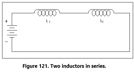
Inductors in Parallel

When two inductors are connected in parallel as shown in Figure 122, each must have the same potential difference between the terminals. When inductors are connected in parallel, the total inductance is less than the smallest inductance. The general equation for n number of inductors in parallel is:

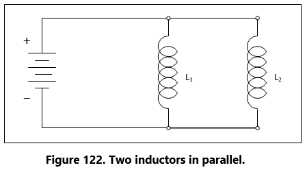
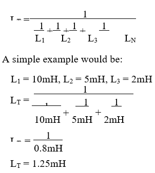
Inductive Reactance

Alternating current is in a constant state of change; the effects of the magnetic fields are a continuously inducted voltage opposition to the current in the circuit. This opposition is called inductive reactance, symbol- ized by XL, and is measured in ohms just as resistance is measured. Inductance is the property of a circuit  to oppose any change in current and is measured in henries. Inductive reactance is a measure of how much the countering emf in the circuit will oppose current variations.

The inductive reactance of a component is directly proportional to the inductance of the component and the applied frequency to the circuit. By increasing either the inductance or applied frequency, the inductive reactance will likewise increase and present more opposition to current in the circuit. This relationship is given as:

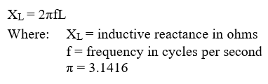
In Figure 123, an AC series circuit is shown in  which the inductance is 0.146 henry and the voltage is 110 volts at a frequency of 60 cycles per second. Inductive reactance is determined by the following method.

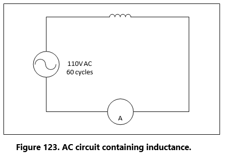
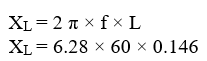
To find current:

In any circuit where there is only resistance, the expression for the relationship of voltage and current is given by Ohm’s law: I = E/ R. Similarly, when there is inductance in an AC circuit, the relationship between voltage and current can be expressed as:

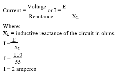
In AC series circuits, inductive reactances are added like resistances in series in a DC circuit. [Figure 124] Thus, the total reactance in the illustrated circuit equals the sum of the individual reactances.

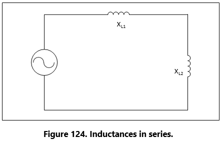
The total reactance of inductors connected in parallel is found the same way as the total resistance in a par- allel circuit. [Figure 125] Thus, the total reactance of inductances connected in parallel, as shown, is expressed as

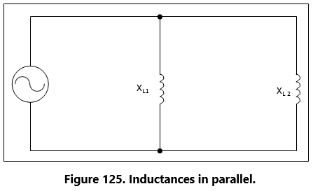
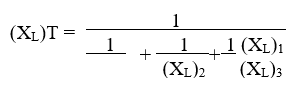
Chapter: 13 AC Circuits

Ohm’s Law for AC Circuits

The rules and equations for DC circuits apply to AC circuits only when the circuits contain resistance alone, as in the case of lamps and heating elements. In order to use effective values of voltage and current in AC circuits, the effect of inductance and capacitance with resistance must be considered.

The combined effects of resistance, inductive reac- tance, and capacitive reactance make up the total opposition to current flow in an ACcircuit. This total opposition is called impedance and is represented by the letter Z. The unit for the measurement of imped- ance is the ohm.

Series AC Circuits

If an AC circuit consists of resistance only, the value of the impedance is the same as the resistance, and Ohm’s law for an AC circuit, I = E/ Z, is exactly the same as for a DC circuit. In Figure 126 a series circuit contain-ing a lamp with 11 ohms resistance connected across a source is illustrated. To find how much current will flow if 110 volts DCis applied and how much current will flow if 110 volts AC are applied, the following examples are solved:

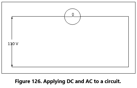
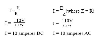
When AC circuits contain resistance and either induc- tance or capacitance, the impedance, Z, is not the same as the resistance, R. The impedance of a circuit is the circuit’s total opposition to the flow of current. In an AC circuit, this opposition consists of resistance and reactance, either inductive or capacitive or elements of both.

Resistance and reactance cannot be added directly, but they can be considered as two forces acting at right angles to each other. Thus, the relation between resistance, reactance, and impedance may be illustrated by a right triangle. [Figure 127]

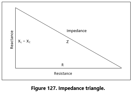
Since these quantities may be related to the sides of a right triangle, the formula for finding the impedance, or total opposition to current flow in an ACcircuit, can be found by using the law of right triangles. This theorem, called the Pythagorean theorem, applies to any right triangle. It states that the square of the hypotenuse is equal to the sum of the squares of the other two sides. Thus, the value of any side of a right triangle can be found if the other two sides are known. If an AC circuit contains resistance and inductance, as shown in Figure 128, the relation between the sides can be stated as:

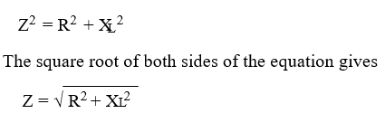
This formula can be used to determine the impedance when the values of inductive reactance and resistance are known. It can be modified to solve for impedance in circuits containing capacitive reactance and resistance by substituting XC in the formula in place of XL. In circuits containing resistance with both inductive and capacitive reactance, the reactances can be combined, but because their effects in the circuit are exactly opposite, they are combined by subtraction:

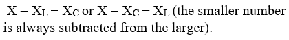
In Figure 128, a series circuit consisting of resistance and inductance connected in series is connected to a source of 110 volts at 60 cycles per second. The resistive element is a lamp with 6 ohms resistance, and the inductive element is a coil with an inductance of 0.021 henry. What is the value of the impedance and the current through the lamp and the coil?

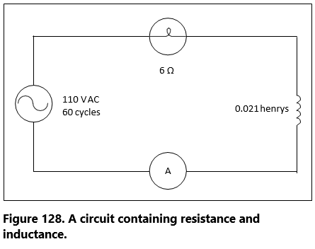
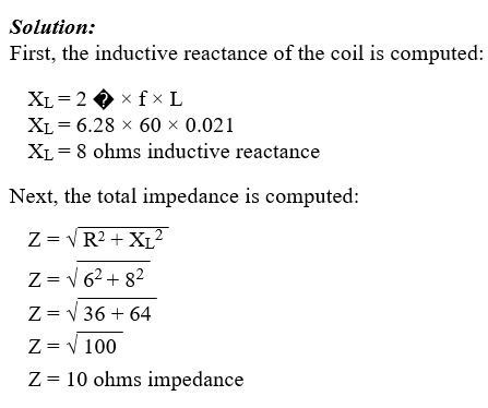
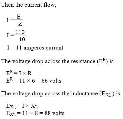
The sum of the two voltages is greater than the impressed voltage. This results from the fact that the two voltages are out of phase and, as such, represent the maximum voltage. If the voltage in the circuit is measured by a voltmeter, it will be approximately 110 volts, the impressed voltage. This can be proved by the equation,

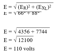
In Figure 129, a series circuit is illustrated in which a capacitor of 200 µf is connected in series with a 10 ohm lamp. What is the value of the impedance, the current flow, and the voltage drop across the lamp?

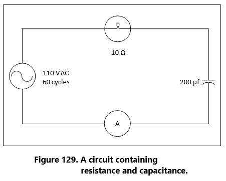
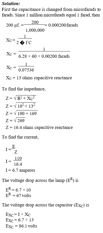
The sum of these two voltages does not equal the applied voltage, since the current leads the voltage. To find the applied voltage,

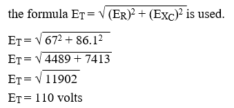
When the circuit contains resistance, inductance, and capacitance, the equation

is used to find the impedance.

Example: What is the impedance of a series circuit, consisting of a capacitor with a reactance of 7 ohms, an inductor with a reactance of 10 ohms, and a resistor with a resistance of 4 ohms? [Figure 130]

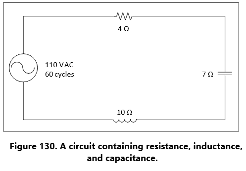
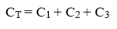
Assuming that the reactance of the capacitor is 10 ohms and the reactance of the inductor is 7 ohms, then XC is greater than XL. Thus,

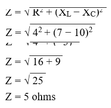
Parallel AC Circuits

The methods used in solving parallel AC circuit prob- lems are basically the same as those used for series AC circuits. Out of phase voltages and currents can be added by using the law of right triangles. However, in solving circuit problems, the currents through the branches are added since the voltage drops across the various branches are the same and are equal to the applied voltage. In Figure 131, a parallel AC circuit containing an inductance and a resistance is shown schematically. The current flowing through the inductance, IL, is 0.0584 ampere, and the current flowing through the resistance is 0.11 ampere. What is the total current in the circuit?

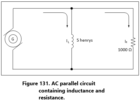
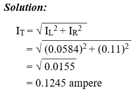
Since inductive reactance causes voltage to lead the current, the total current, which contains a component of inductive current, lags the applied voltage. If the current and voltages are plotted, the angle between the two, called the phase angle, illustrates the amount the current lags the voltage.

In Figure 132, a 110-volt generator is connected to a load consisting of a 2 µf capacitance and a 10,000- ohm resistance in parallel. What is the value of the impedance and total current flow?

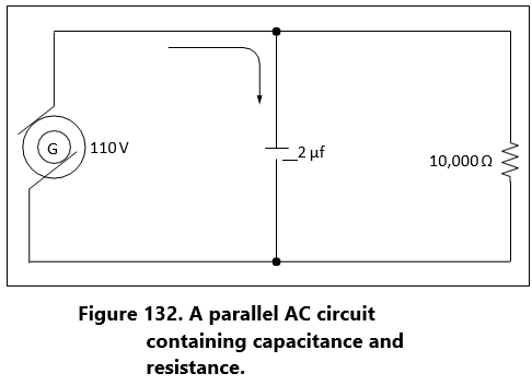
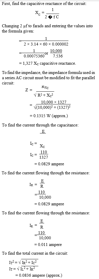
Resonance

It has been shown that both inductive reactance (XL = 2 � f L) and capacitive reactance:

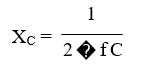
…are functions of an alternating current frequency. Decreasing the frequency decreases the ohmic value of the inductive reactance, but a decrease in frequency increases the capacitive reactance. At some particular frequency, known as the resonant frequency, the reactive effects of a capacitor and an inductor will  be equal. Since these effects are the opposite of one another, they will cancel, leaving only the ohmic value of the resistance to oppose current flow in a circuit. If the value of resistance is small or consists only of the resistance in the conductors, the value of current flow can become very high.

In a circuit where the inductor and capacitor are in series, and the frequency is the resonant frequency, or frequency of resonance, the circuit is said to be “in resonance” and is referred to as a series resonant circuit. The symbol for resonant frequency is Fn.

If, at the frequency of resonance, the inductive reac- tance is equal to the capacitive reactance, then:

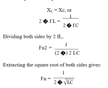
Where Fn is the resonant frequency in cycles per second, C is the capacitance in farads, and L is the inductance in henries. With this formula, the frequency at which a capacitor and inductor will be resonant can be determined.

To find the inductive reactance of a circuit use:

The impedance formula used in a series AC circuit must be modified to fit a parallel circuit.

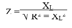
To find the parallel networks of inductance and capacitive reactors, use:

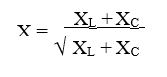
To find the parallel networks with resistance capacitive and inductance, use:

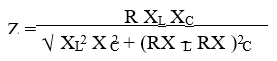
Since at the resonant frequency XL cancels XC, the cur- rent can become very large, depending on the amount of resistance. In such cases, the voltage drop across the inductor or capacitor will often be higher than the applied voltage.

In a parallel resonant circuit, the reactances are equal and equal currents will flow through the coil and the capacitor. [Figure 133]

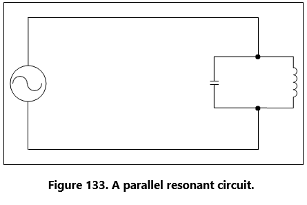
Since the inductive reactance causes the current through the coil to lag the voltage by 90°, and the capacitive reactance causes the current through the capacitor to lead the voltage by 90°, the two currents are 180° out of phase. The canceling effect of such currents would mean that no current would flow from the generator and the parallel combination of the inductor, and the capaci- tor would appear as infiniteimpedance. In practice, no such circuit is possible, since some value of resistance is always present, and the parallel circuit, sometimes called a tank circuit, acts as very high impedance. It is also called an antiresonant circuit, since its effect in a circuit is opposite to that of a series resonant circuit, in which the impedance is very low.

Power in AC Circuits

In a DC circuit, power is obtained by the equation, P = EI, (watts equal volts times amperes). Thus, if 1 ampere of current flows in a circuit at a pressure of 200 volts, the power is 200 watts. The product of the volts and the amperes is the true power in the circuit.

True Power Defined

The power dissipated in the resistance of a circuit, or the power actually used in the circuit.

In an AC circuit, a voltmeter indicates the effective voltage and an ammeter indicates the effective cur- rent. The product of these two readings is called the apparent power.

Apparent Power Defined

That power apparently available for use in an AC circuit containing a reactive component. It is the product of effective voltage times the effective current, expressed in volt-amperes. It must be multiplied by the power factor to obtain true power available.

Only when the AC circuit is made up of pure resistance is the apparent power equal to the true power. [Figure 134] When there is capacitance or inductance in the circuit, the current and voltage are not exactly in phase, and the true power is less than the apparent power. The true power is obtained by a wattmeter reading. The ratio of the true power to the apparent power is called the power factor and is usually expressed in percent. In equation form, the relationship is:

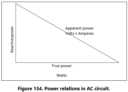
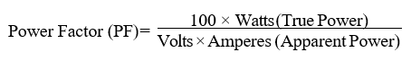
Example: A 220-volt AC motor takes 50 amperes from the line, but a wattmeter in the line shows that only 9,350 watts are taken by the motor. What are the apparent power and the power factor?

Transformers

A transformer changes electrical energy of a given voltage into electrical energy at a different voltage level. It consists of two coils that are not electrically connected, but are arranged so that the magnetic field surrounding one coil cuts through the other coil. When an alternating voltage is applied to (across) one coil, the varying magnetic field set up around that coil cre- ates an alternating voltage in the other coil by mutual induction. A transformer can also be used with pulsat- ing DC, but a pure DC voltage cannot be used, since only a varying voltage creates the varying magnetic field that is the basis of the mutual induction process.

A transformer consists of three basic parts. [Figure 135] These are an iron core which provides a circuit of low reluctance for magnetic lines of force, a primary winding which receives the electrical energy from the source of applied voltage, and a secondary winding which receives electrical energy by induction from the primary coil.

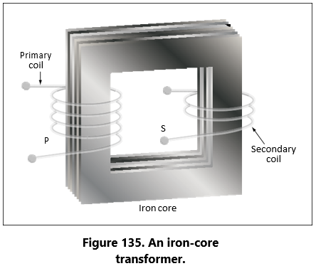
The primary and secondary of this closed core trans- former are wound on a closed core to obtain maximum inductive effect between the two coils.

There are two classes of transformers: (1) voltage transformers used for stepping up or stepping down voltages, and (2) current transformers used in instru- ment circuits.

In voltage transformers, the primary coils are con- nected in parallel across the supply voltage as shown in Figure 136A. The primary windings of current transformers are connected in series in the primary circuit [Figure 136B]. Of the two types, the voltage transformer is the more common.

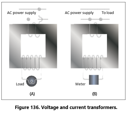
There are many types of voltage transformers. Most of these are either step-up or step-down transformers. The factor that determines whether a transformer is  a step-up, or step-down type is the “turns” ratio. The turns ratio is the ratio of the number of turns in the pri- mary winding to the number of turns in the secondary winding. For example, the turns ratio of the step- down transformer shown in Figure 137A is 5 to 1, since there are five times as many turns in the primary as in the secondary. The step-up transformer shown in Figure 137B has a 1 to 4 turns ratio.

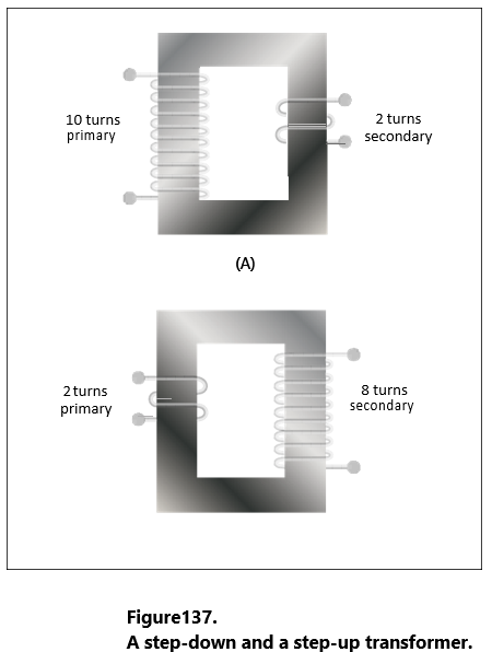
The ratio of the transformer input voltage to the output voltage is the same as the turns ratio if the transformer is 100 percent efficient. Thus, when 10 volts are applied to the primary of the transformer shown in Figure 137A, two volts are induced in the  secondary. If 10 volts are applied to the primary of the transformer in Figure 137B, the output voltage across the terminals of the secondary will be 40 volts.

No transformer can be constructed that is 100 percent efficient, although iron core transformers can approach this figure. This is because all the  magnetic lines of force set up in the primary do not cut across the turns of the secondary coil. A certain amount of the magnetic flux, called leakage flux, leaks out of the magnetic circuit. The measure of how well the flux of the primary is coupled into the secondary is called the “coefficient of coupling.” For example, if it is assumed that the primary of a transformer develops 10,000 lines of force and only 9,000 cut across the secondary, the coefficient of coupling would be 0.9 or, stated another way, the transformer would be 90 percent efficient.

When an AC voltage is connected across the primary terminals of a transformer, an alternating current will flow and self induce a voltage in the primary coil that is opposite and nearly equal to the applied voltage. The difference between these two voltages allows just enough current in the primary to magnetize its core. This is called the exciting, or magnetizing, current. The magnetic field caused by this exciting current cuts across the secondary coil and induces a voltage by mutual induction.

If a load is connected across the secondary coil, the load current flowing through the secondary coil will produce a magnetic field which will tend to neutralize the magnetic field produced by the primary current. This will reduce the self-induced (opposition) voltage in the primary coil and allow more primary current to flow. The primary current increases as the secondary load current increases, and decreases as the secondary load current decreases. When the secondary load is removed, the primary current is again reduced to the small exciting current sufficient only to magnetize the iron core of the transformer.

If a transformer steps up the voltage, it will step down the current by the same ratio. This should be evident if the power formula is considered, for the power (I × E) of the output (secondary) electrical energy is the same as the input (primary) power minus that energy loss in the transforming process. Thus, if 10 volts and 4 amps (40 watts of power) are used in the primary to produce a magnetic field, there will be 40 watts of power developed in the secondary (disregarding any loss). If the transformer has a step-up ratio of 4 to 1, the voltage across the secondary will be 40 volts and the current will be 1 amp. The voltage is 4 times greater and the current is one-fourth the primary circuit value, but the power (I × E value) is the same.

When the turns ratio and the input voltage are known, the output voltage can be determined as follows:

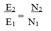
Where E is the voltage of the primary, E2 is the output voltage of the secondary, and N1 and N2 are the number of turns of the primary and secondary, respectively.

Transposing the equation to find the output voltage gives:

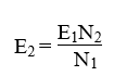
The most commonly used types of voltage transformers are as follows:

1. Power transformers are used to step up or step down voltages and current in many types of power supplies. They range in size from the small power transformer shown in Figure 138 used in a radio receiver to the large transformers used to step down high power line voltage to the 110 – 120 volt level used in homes. Figure 139 shows the schematic symbol for an iron core transformer. In this case, the secondary is made up of three separate windings. Each winding supplies a different circuit with a specific voltage, which saves the weight, space, and expense of three separate transformers. Each secondary has a midpoint connection, called a “center tap,” which provides a selection of half the voltage across the whole winding. The leads from the various windings are color coded by the manufacturer, as labeled in Figure 139. This is a standard color code, but other codes or numbers may be used.
   
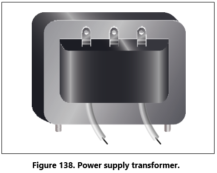
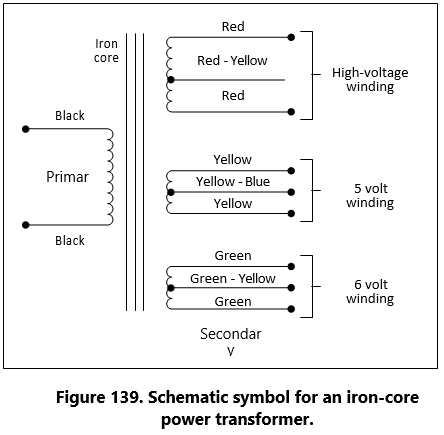
2. Audio transformers resemble power They have only one secondary and are designed to operate over the range of audio frequencies (20 to 20,000 cps).
3. RF transformers are designed to operate in equipment that functions in the radio range of frequencies. The symbol for the RF transformer is the same as for an RF choke coil. It has an air core as shown in Figure 140
   
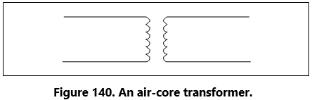
4. Autotransformers are normally used in power circuits; however, they may be designed for other uses. Two different symbols for autotransformers used in power or audio circuits are shown in Figure 141. If used in an RF communication or navigation circuit (Figure 141B), it is the same, except there is no symbol for an iron core. The autotransformer uses part of a winding as a primary; and, depending on whether it is step up or step down, it uses all or part of the same winding as the secondary. For example, the autotransformer shown in Figure 141A could  use the following possible choices for primary and secondary terminals.
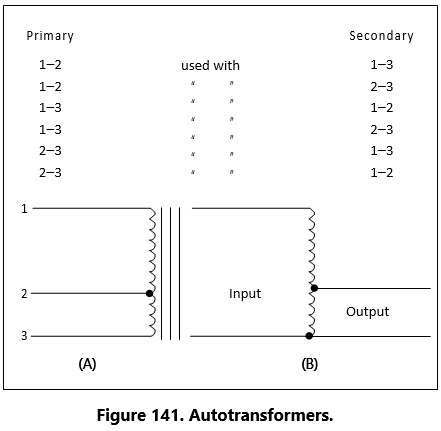   Current TransformersCurrent transformers are used in AC power supply systems to sense generator line current and to provide a current, proportional to the line current, for circuit protection and control devices.The current transformer is a ring-type transformer using a current carrying power lead as a primary (either the power lead or the ground lead of the AC genera- tor). The current in the primary induces a current in the secondary by magnetic induction.The sides of all current transformers are marked “H1” and “H2” on the unit base. The transformers must be installed with the “H1” side toward the generator in the circuit in order to have proper polarity. The sec- ondary of the transformer should never be left open while the system is being operated; to do so couldcause dangerously high voltages, and could overheat the transformer. Therefore, the transformer output con- nections should always be connected with a jumper when the transformer is not being used but is left in the system.Transformer LossesIn addition to the power loss caused by imperfect cou- pling, transformers are subject to “copper” and “iron” losses. The resistance of the conductor comprising the turns of the coil causes copper loss. The iron losses are of two types called hysteresis loss and eddy current loss. Hysteresis loss is the electrical energy required to magnetize the transformer core, first in one direction and then in the other, in step with the applied alternat- ing voltage. Eddy current loss is caused by electric currents (eddy currents) induced in the transformer core by the varying magnetic fields. To reduce eddy current losses, cores are made of laminations coated with an insulation, which reduces the circulation of induced currents.Power in TransformersSince a transformer does not add any electricity to the circuit but merely changes or transforms the electricity that already exists in the circuit from one voltage to another, the total amount of energy in a circuit must remain the same. If it were possible to construct a perfect transformer, there would be no loss of power in it; power would be transferred undiminished from one voltage to another.

   Since power is the product of volts times amperes, an increase in voltage by the transformer must result in a decrease in current and vice versa. There cannot be more power in the secondary side of a transformer than there is in the primary. The product of amperes times volts remains the same.

   The transmission of power over long distances is accomplished by using transformers. At the power source, the voltage is stepped up in order to reduce the line loss during transmission. At the point of utilization, the voltage is stepped down, since it is not feasible to use high voltage to operate motors, lights, or other electrical appliances.

   Chapter: 14 DC Measuring Instruments

   Understanding the functional design and operation of electrical measuring instruments is very important, since they are used in repairing, maintaining, and troubleshooting electrical circuits. The best and most expensive measuring instrument is of no use unless the technician knows what is being measured and what each reading indicates. The purpose of the meter is to measure quantities existing in a circuit. For this reason, when a meter is connected to a circuit, it must not change the characteristics of that circuit.

   Meters are either self-excited or externally excited. Those that are self-excited operate from a power source within the meter. Externally excited meters get their power source from the circuit that they are connected to. The most common analog meters in use today are the voltmeter, ammeter, and ohmmeter. All of which operate on the principles of electromagnetism. The fundamental principle behind the operation of the meter is the interaction between magnetic fields created by a current gathered from the circuit in some manner. This interaction is between the magnetic fields of a permanent magnet and the coils of a rotating magnet. The greater the current through the coils of the rotat- ing magnet, the stronger the magnetic field produced. A stronger field produces greater rotation of the coil. While some meters can be used for both DC and AC circuit measurement, only those used as DC instru- ments are discussed in this section. The meters used for AC, or for both AC and DC, are discussed in the study of AC theory and circuitry.

   D’Arsonval Meter Movement

   This basic DC type of meter movement — first employed by the French scientist, d’Arsonval in mak- ing electrical measurement— is a current measuring device, which is used in the ammeter, voltmeter, and ohmmeter. The pointer is deflected in proportion to the amount of current through the coil. Basically, both the ammeter and the voltmeter are current measuring instruments, the principal difference being the method in which they are connected in a circuit. While an ohm- meter is also basically a current measuring instrument, it differs from the ammeter and voltmeter in that it provides its own source (self-excited) of power and contains other auxiliary circuits.

   Current Sensitivity and Resistance

   The current sensitivity of a meter movement is the amount of current required to drive the meter move- ment to a full-scale deflection. A simple example would be a meter movement that has 1mA sensitivity. What this indicates is that meter movement will require 1mA of current to move the needle to a full-scale indica- tion. Likewise a half scale deflection will require only 0.5mA of current. Additionally, what is called move- ment resistance is the actual DC resistance of the wire used to construct the meter coil.

   In a standard d’Arsonval meter movement may have a current sensitivity of 1mA and a resistance of 50Ω. If the meter is going to be used to measure more than 1mA then additional circuitry will be required to accomplish the task. This additional circuitry is a simple shunt resistor. The purpose of the shunt resistor is to bypass current that exceeds the 1mA limitation of the meter movement. To illustrate this, assume that the 1mA meter in question is needed to measure 10mA. The shunt resistor used should carry 9mA while the remaining 1mA is allowed to pass through the meter. [Figure 142]

   

   

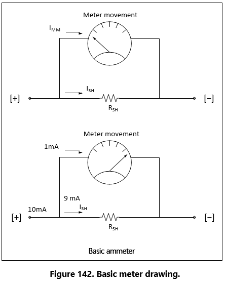
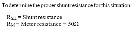
   Because the shunt resistance and the 50Ω meter resis- tance are in parallel, the voltage drop across both of them is the same.

   

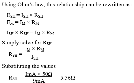
   Damping

   To make meter readings quickly and accurately, it is desirable that the moving pointer overshoot its proper position only a small amount and come to rest after not more than one or two small oscillations. The term “damping” is applied to methods used to bring the pointer of an electrical meter to rest after it has been set in motion. Damping may be accomplished by electrical means, by mechanical means, or by a combination of both.

   Electrical Damping

   A common method of damping by electrical means is to wind the moving coil on an aluminum frame. As the coil moves in the field of the permanent magnet, eddy currents are set up in the aluminum frame. The magnetic field produced by the eddy currents opposes the motion of the coil. The pointer will therefore swing more slowly to its proper position and come to rest quickly with very little oscillation.

   Mechanical Damping

   Air damping is a common method of damping by mechanical means. As shown in Figure 143, a vane is attached to the shaft of the moving element and enclosed in an air chamber. The movement of the shaft is retarded because of the resistance that the air offers to the vane. Effective damping is achieved if the vane nearly touches the walls of the chamber.

   

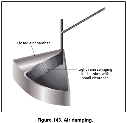
   A Basic Multirange Ammeter

   Building upon the basic meter previously discussed is the more complex and useful multirange meter, which is more practical. The basic idea of a multirange ammeter is to make the meter usable over a wide range of voltages. In order to accomplish this, each range must utilize a different shunt resistance. The example give in this text is that of a two-range meter. However, once the basics of a two range multirange ammeter are understood, the concepts can easily be transferred to the design of meters with many selectable ranges.

   Figure 144 shows the schematic of an  ammeter  with two selectable ranges. This example builds upon the previous 10mA range meter by adding a 100mA range. With the switch selected to the 10mA range, the meter will indicate 10mA when the needle is deflected to full scale and will likewise indicate 100mA at full scale when selected to 100mA.

   

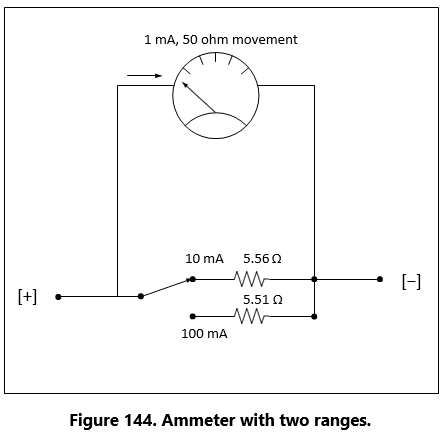
   The value of the 100mA shunt resistor is determined the same way the 10mAshunt resistor was determined. Recall that the meter movement can only carry 1mA.

   This means that in a 100mA range the remaining cur- rent of 99mA must pass through the shunt resistor.

   

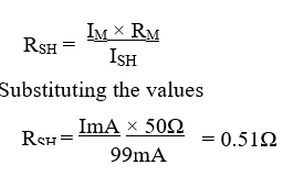
   Precautions

   The precautions to observe when using an ammeter are summarized as follows:

   1. Always connect an ammeter in series with the element through which the current flow is to be measured.
   2. Never connect an ammeter across a source of voltage, such as a battery or Remember that the resistance of an ammeter, particularly on the higher ranges, is extremely low and that any voltage, even a volt or so, can cause very high current to flow through the meter, causing damage to it.
   3. Use a range large enough to keep the deflection less than full scale. Before measuring a current, form some idea of its magnitude. Then switch  to a large enough scale or start with the highest range and work down until the appropriate scale is reached. The most accurate readings are obtained at approximately half-scale deflection. Many milliammeters have been ruined by attempts to measure amperes. Therefore, be sure to read the lettering either on the dial or on the switch positions and choose proper scale before connecting the meter in the circuit.
   4. Observe proper polarity in connecting the meter in the circuit. Current must flow through the coil in a definite direction in order to move the indicator needle up Current reversal because of incorrect connection in the circuit results in a reversed meter deflection and frequently causes bending of the meter needle. Avoid improper meter connections by observing the polarity markings on the meter.

   The Voltmeter

   The voltmeter uses the same type of meter movement as the ammeter but employs a different circuit external to the meter movement.

   As shown before, the voltage drop across the meter coil is a function of current and the coil resistance. In another example, 50μA × 1000Ω = 50mV. In order for the meter to be used to measure voltages greater than 50mV, there must be added a series resistance to drop any excess voltage greater than that which the meter movement requires for a full scale deflection. The case of the voltmeter, this resistance is called multiplier resistance and will be designated as RM. Figure 145 illustrates a basic voltmeter. This voltmeter only has one multiplier resistor for use in one range. In this example, the full scale reading will be 1 volt. RM is determined in the follow way:

   The meter movement drops 50mV at a full scale deflection of 50μA. The multiplying resistor RMmust drop the remaining voltage of 1V − 50mV = 950 mV. Since RM is in series with the movement, it also carries 50μA at full scale.

   

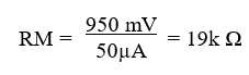
   Therefore, for 1 volt full scale deflection, the total resis- tance of the voltmeter is 20 k Ω. That is, the multiplier resistance and the coil resistance.

   Voltmeter Sensitivity

   Voltmeter sensitivity is defined in terms of resistance per volt (Ω/ V). The meter used in the previous example has a sensitivity of 20 k Ωand a full scale deflection of 1 volt.

   Multiple Range Voltmeters

   The simplified voltmeter in Figure 145 has  only  one range (1 volt), which means that it can measure voltages from 0 volts to 1 volt. In order for the meter to be more useful, additional multiplier resistors must be used. One resistor must be used for each desired range.

   

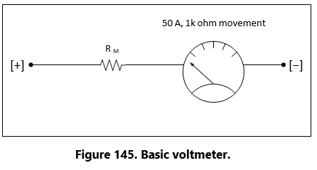
   For a 50μA movement, the total resistance required is 20 k Ωfor each volt of full scale reading. In other words, the sensitivity for a 50μA movement is always 20 k Ωregardless of the selected range. The full-scale meter current is 50μA at any range selection. To find the total meter resistance, multiply the sensitivity by the full scale voltage for that particular range. For example for a 10 volt range, RT = (20k Ω/ V)/(10 V) = 200k Ω.The total resistance for the 1 volt range is 20k Ω,so RMfor a 10 V range will be 200k Ω− 20k Ω = 180k Ω. This two-range voltmeter is illustrated in Figure 146.

   

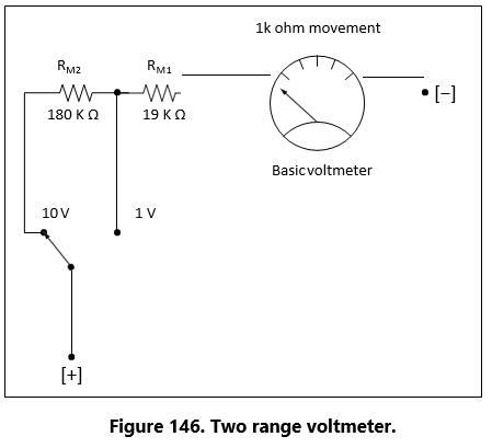
   Voltmeter Circuit Connections

   When voltmeters are used, they are connected in parallel with a circuit. If unsure about the voltage to be measured, take the first reading at the high value on the meter and then progressively move down through the range until a suitable read is obtained. Observe that the polarity is correct before connecting the meter to the circuit or damage will occur by driving the movement backwards.

   Influence of the Voltmeter in the Circuit

   When a voltmeter is connected across two points in  a circuit, current will be shunted. If the voltmeter has low resistance, it will draw off a significant amount of current. This will lower the effective resistance of the circuit and change the voltage readings. When making a voltage measurement, use a high resistance voltmeter to prevent shunting of the circuit.

   The Ohmmeter

   The meter movement used for the ammeter and the voltmeter can also be used for the ohmmeter. The function of the ohmmeter is to measure resistance. A simplified one-stage ohmmeter is illustrated in Figure 147, which shows that the basic ohmmeter contains a battery and a variable resistor in series with the  meter movement. To measure resistance, the leads of the meter are connected across an external resistance, which is to be measured. By doing this the ohmmeter circuit is completed. This connection allows the inter- nal battery to produce a current through the movement coil, causing a deflection of the pointer proportional to the value of the external resistance being measured.

   

   Zero Adjustment

   When the ohmmeter leads are open as shown in Figure 148, the meter is at a full scale deflection, indicating an infinite (∞) resistance or an open circuit. Whenthe leads are shorted as shown in figure “zero adjust,” the pointer will be at the full right hand position, indicating a short circuit or zero resistance. The purpose of the variable resistor in this figure is to adjust the current so that the pointer is at exactly zero when the leads are shorted. This is used to compensate for changes in the internal battery voltage due to aging.

   

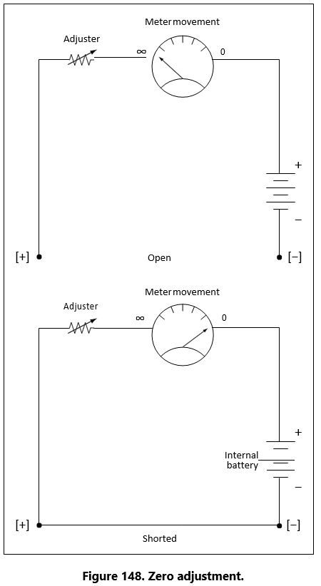
   Ohmmeter Scale

   Figure 149 shows a typical analog ohmmeter scale. Between zero and infinity (∞), the scale is marked to indicate various resistor values. Because the values decrease from left to right, this scale is often called a back-off scale.

   

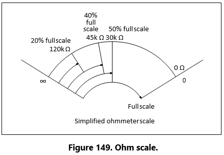
   In the case of the example given, assume that a certain ohmmeter uses a 50μA, 1000Ωmeter movement and has an internal 1.5 volt battery. A current of 50μA produces a full-scale deflection when the test leads are shorted. To have 50μA, the total ohmmeter resis- tance is 1.5 V/50μA = 30kΩ.Therefore, since the coil resistance is 1kΩ, the variable zero adj ustment resistor must be set to 30kΩ – 1kΩ = 29kΩ.

   Now consider that a 120kΩresistor is connected to the ohmmeter leads. Combined with the 30kΩ internal resistance, the total Ris 150kΩ. The current is 1.5 V/150kΩ= 10μA, which is 20% of the full scale cur- rent and which appears on the scale as shown in Figure 149.

   Now consider further that a 120kΩresistor is connected to the ohmmeter leads. This will result in a current of 1.5V/75kΩ = 10μA, which is 40% of the full scale current and which is marked on the scale as shown. Additional calculations of this type show that the scale is nonlinear. It is more compressed toward the left side than the right side. The center scale point corresponds to the internal meter resistance of 30kΩ. The reason is as follows:

   With  30kΩconnected  to  the  leads,  the  current  is 1.5V/60kΩ= 25μA, which is half of the full scale current of 50μA.

   The Multirange Ohmmeter

   A practical ohmmeter usually has several operational ranges. These typically are indicated by R × 1, R × 10, R × 100, R × 1k, R × 100k and R × 1M. These range selections are interpreted in a different manner than that of an ammeter or voltmeter. The reading on the ohmmeter scale is multiplied by the factor indicated by the range setting. For example, if the pointer is set on the scale and the range switch is set at R × 100, the actual resistance measurement is 20 × 100 or 2kΩ.

   To measure small resistance values, the technician must use a higher ohmmeter current than is needed for measuring large resistance values. Shunt resistors are needed to provide multiple ranges on the ohmmeter to measure a range of resistance values from the very small to very large. For each range, a different value of shunt resistance is switched in. The shunt resistance increases for higher ohm ranges and is always equal to the center scale reading on any selected range. In some meters, a higher battery voltage is used for the highest ohm range. A common circuit arrangement is shown in Figure 150.

   

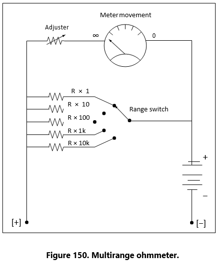
   Megger (Megohmmeter)

   The megger, or megohmmeter, is a high range ohm- meter containing a hand-operated generator. It is used to measure insulation resistance and other high resis- tance values. It is also used for ground, continuity, and short circuit testing of electrical power systems. The chief advantage of the megger over an ohmmeter is its capacity to measure resistance with a high potential, or “breakdown” voltage. This type of testing ensures that insulation or a dielectric material will not short or leak under potential electrical stress.

   The megger consists of two primary elements, both of which are provided with individual magnetic fields from a common permanent magnet: (1) a hand-driven DC generator, G, which supplies the necessary current for making the measurement, and (2) the instrument portion, which indicates the value of the resistance being measured. The instrument portion is of the opposed coil type. Coils A and B are mounted on the movable member with a fixed angular relationship to each other and are free to turn as a unit in a magnetic field. CoilB tends to move the pointer counterclock- wise and coil A, clockwise. The coils are mounted on a light, movable frame that is pivoted in jewel bearings and free to move about axis 0. [Figure 151]

   

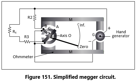
   Coil A is connected in series with R3 and the unknown resistance, Rx, to be measured. The series combination of coil A, R3, and Rx is connected between the + and brushes of the DC Coil B is connected in series with R2 and this combination is also connected across the generator. There are no restraining springs on the movable member of the instrument portion of the megger. When the generator is not in operation, the pointer floats freely and may come to rest at any position on the scale.

   If the terminals are open circuited, no current flows in coil A, and the current in coil B alone controls the movement of the moving element. Coil B takes a position opposite the gap in the core (since the core cannot move and coil B can), and the pointer indicates infinity on the scale. When a resistance is connected between the terminals, current flows in coil A, tending to move the pointer clockwise. At the same time, coil B tends to move the pointer counterclockwise. There- fore, the moving element, composed of both coils and the pointer, comes to rest at a position at which the two forces are balanced. This position depends upon the value of the external resistance, which controls the relative magnitude of current of coil A. Because changes in voltage affect both coils A and B in the same proportion, the position of the moving element is independent of the voltage. If the terminals are short circuited, the pointer rests at zero because the current in A is relatively large. The instrument is not dam- aged under these circumstances because the current is limited by R3.

   There are two types of hand-driven meggers: the variable type and the constant pressure type. The speed of the variable pressure megger is dependent on how fast the hand crank is turned. The constant pressure megger uses a centrifugal governor, or slip clutch. The governor becomes effective only when the megger is operated at a speed above its slip speed, at which speed its voltage remains constant.

   Chapter: 15 AC Measuring Instruments

   A DC meter, such as an ammeter, connected in an AC circuit will indicate zero, because the meter movements used in a d’Arsonval type movement is restricted to direct current. Since the field of a permanent magnet in the d’Arsonval type meter remains constant and in the same direction at all times, the moving coil fol- lows the polarity of the current. The coil attempts to move in one direction during half of the AC cycle and in the reverse direction during the other half when the current reverses.

   The current reverses direction too rapidly for the coil to follow, causing the coil to assume an average position. Since the current is equal and opposite during each half of the AC cycle, the direct current meter indicates zero, which is the average value. Thus, a meter with a permanent magnet cannot be used to measure alter- nating voltage and current. For AC measurements of current and voltage, additional circuitry is required. The additional circuitry has a rectifier, which converts ACto DC. There are two basic types of rectifiers: One is the half-wave rectifier and the other is the full-wave rectifier. Both of these are depicted in block diagram form in Figure 152.

   

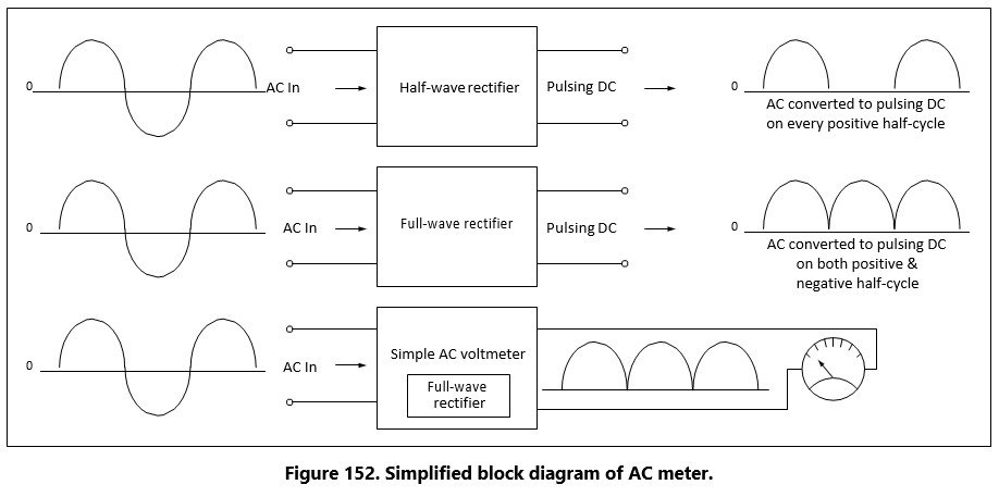
   Figure 152 also shows a simplified block diagram of an ACmeter. In this depiction, the full-wave rectifier precedes the meter movement. The movement responds to the average value of the pulsating DC. The scale can then be calibrated to show anything the designer wants. In most cases, it will be root mean square (RMS) value or peak value.

   Electrodynamometer Meter Movement

   The electrodynamometer can be used to measure alter- nating or direct voltage and current. It operates on the same principles as the permanent magnet moving coil meter, except that the permanent magnet is replaced by an air core electromagnet. The field of the electrodyna- mometer is developed by the same current that flows through the moving coil. [Figure 153]

   

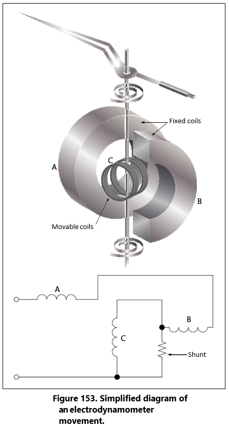
   Because this movement contains no iron, the elec- trodynamometer can be used as a movement for both AC and DC instruments. Alternating current can be measured by connecting the stationary and moving coils in series. Whenever the current in the moving coil reverses, the magnetic field produced by the stationary coil reverses. Regardless of the direction of the current, the needle will move in a clockwise direction.

   However, for either voltmeter or ammeter applications, the electrodynamometer is too expensive to economi- cally compete with the d’Arsonval type movement.

   Moving Iron Vane Meter

   The moving iron vane meter is another basic type of meter. It can be used to measure either AC or DC. Unlike the d’Arsonval meter, which employs perma- nent magnets, it depends on induced magnetism for its operation. It utilizes the principle of repulsion between two concentric iron vanes, one fixed and one movable, placed inside a solenoid. A pointer is attached to the movable vane. [Figure 154]

   

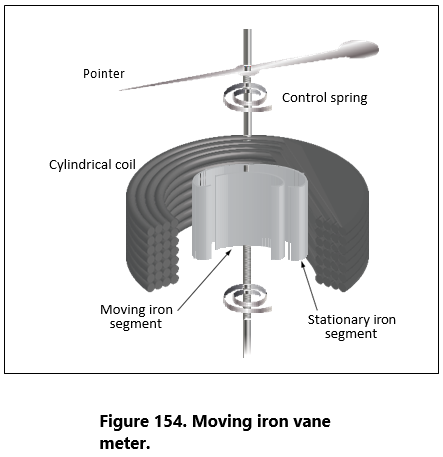
   When current flows through the coil, the two iron vanes become magnetized with north poles at their upper ends and south poles at their lower ends for one direction of current through the coil. Because like poles repel, the unbalanced component of force, tangent to the movable element, causes it to turn against the force exerted by the springs.

   The movable vane is rectangular in shape and the fixed vane is tapered. This design permits the use of a relatively uniform scale.

   When no current flows through the coil, the movable vane is positioned so that it is opposite the larger portion of the tapered fixed vane, and the scale reading is zero. The amount of magnetization of the vanes depends on the strength of the field, which, in turn, depends on the amount of current flowing through the coil.

   The force of repulsion is greater opposite the larger end of the fixed vane than it is nearer the smaller end. Therefore, the movable vane moves toward the smaller end through an angle that is proportional to the magnitude of the coil current. The movement ceases when the force of repulsion is balanced by the restraining force of the spring.

   Because the repulsion is always in the same direction (toward the smaller end of the fixed vane), regardless of the direction of current flow through the coil, the moving iron vane instrument operates on either DC or AC circuits.

   Mechanical damping in this type of instrument can be obtained by the use of an aluminum vane attached to the shaft so that, as the shaft moves, the vane moves in a restricted air space.

   When the moving iron vane meter is used as an ammeter, the coil is wound with relatively few turns of large wire in order to carry the rated current.

   When the moving iron vane meter is used as a volt- meter, the solenoid is wound with many turns of small wire. Portable voltmeters are made with self-contained series resistance for ranges up to 750 volts. Higher ranges are obtained by the use of additional external multipliers.

   The moving iron vane instrument may be used to measure direct current but has an error due to residual magnetism in the vanes. Reversing the meter connections and averaging the readings may minimize the error. When used on AC circuits, the instrument has an accuracy of 0.5 percent. Because of its simplicity, relatively low cost, and the fact that no current is conducted to the moving element, this type of movement is used extensively to measure current and voltage in AC power circuits. However, because the reluctance of the magnetic circuit is high, the moving iron vane meter requires much more power to produce full-scale deflection than is required by a d’Arsonval meter of the same range. Therefore, the moving iron vane meter is seldom used in high resistance low power circuits.

   Inclined Coil Iron Vane Meter

   The principle of the moving iron vane mechanism is applied to the inclined coil type of meter, which can be used to measure both AC and DC. The inclined coil, iron vane meter has a coil mounted at an angle to the shaft. Attached obliquely to the shaft, and located inside the coil, are two soft iron vanes. When no cur- rent flows through the coil, a control spring holds the pointer at zero, and the iron vanes lie in planes parallel to the plane of the coil. When current flows through the coil, the vanes tend to line up with magnetic lines passing through the center of the coil at right angles to the plane of the coil. Thus, the vanes rotate against the spring action to move the pointer over the scale.

   The iron vanes tend to line up with the magnetic lines regardless of the direction of current flow through the coil. Therefore, the inclined coil, iron vane meter can be used to measure either alternating current or direct current. The aluminum disk and the drag magnets provide electromagnetic damping.

   Like the moving iron vane meter, the inclined coil type requires a relatively large amount of current for full- scale deflection and is seldom used in high resistance low power circuits.

   As in the moving iron vane instruments, the inclined coil instrument is wound with few turns of relatively large wire when used as an ammeter and with many turns of small wire when used as a voltmeter.

   Varmeters

   Multiplying the volts by the amperes in an AC circuit gives the apparent power: the combination of the true power (which does the work) and the reactive power (which does no work and is returned to the line). Reactive power is measured in units of vars (volt-amperes reactive) or kilovars (kilovolt-amperes reactive, abbreviated kVAR). When properly connected, wattmeters measure the reactive power. As such, they are called varmeters. Figure 155 shows a varmeter connected in an AC circuit.

   

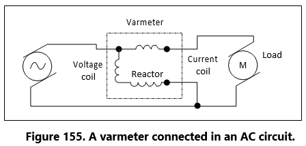
   Wattmeter

   Electric power is measured by means of a wattmeter. Because electric power is the product of current and voltage, a wattmeter must have two elements, one for current and the other for voltage. For this reason, wattmeters are usually of the electrodynamometer type. [Figure 156]

   

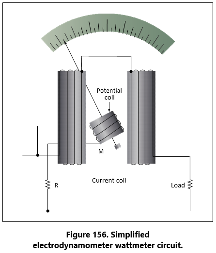
   The movable coil with a series resistance forms the voltage element, and the stationary coils constitute the current element. The strength of the field around the potential coil depends on the amount of current that flows through it. The current, in turn, depends on the load voltage applied across the coil and the high resistance in series with it. The strength of the field around the current coils depends on the amount of current flowing through the load. Thus, the meter deflection is proportional to the product of the volt- age across the potential coil and the current through the current coils. The effect is almost the same (if the scale is properly calibrated) as if the voltage applied across the load and the current through the load were multiplied together.

   If the current in the line is reversed, the direction of current in both coils and the potential coil is reversed, the net result is that the pointer continues to read up scale. Therefore, this type of wattmeter can be used to measure either AC or DC power.

   Frequency Measurement/Oscilloscope

   The oscilloscope is by far one of the more useful electronic measurements available. The viewing capabilities of the oscilloscope make it possible to see and quantify various waveform characteristics such as phase relationships, amplitudes, and durations. While oscilloscopes come in a variety of configurations and presentations, the basic operation is typically the same. Most oscilloscopes in general bench or shop applica- tions use a cathode-ray tube (CRT), which is the device or screen that displays the waveforms.

   The CRT is a vacuum instrument that contains an electron gun, which emits a very narrow and focused beam of electrons. A phosphorescent coat applied to the back of the screen forms the screen. The beam is electronically aimed and accelerated so that the electron beam strikes the screen. When the electron beam strikes the screen, light is emitted at the point of impact.

   Figure 157 shows the basic  components  of  the  CRT with a block diagram. The heated cathode emits electrons. The magnitude of voltage on the control grid determines the actual flow of electrons and thus controls the intensity of the electron beam. The accel- eration anodes increase the speed of the electrons, and the focusing anode narrows the beam down to a fine point. The surface of the screen is also an anode and will assist in the acceleration of the electron beam.

   

   The purpose of the vertical and horizontal deflection plates is to bend the electron beam and position it to a specific point of the screen. Figure 158 illustrates how the deflection plates are used to position the beam on the screen. By providing a neutral or zero voltage to a deflection plate, the electron beam will be unaffected. By applying a negative voltage to a plate, the electron beam with be repelled and driven away from the plate. Finally, by applying a positive voltage, the electron beam will be drawing to the plate. Figure 158 pro- vides a few possible plate voltage combinations and the resultant beam position.

   

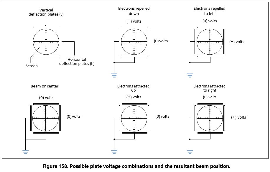
   Horizontal Deflection

   To get a visual representation of the input signal, an internally generated saw-tooth voltage is generated and then applied to the horizontal deflection plates. Figure 159 illustrates that the saw-tooth is a pattern of voltage applied, which begins at a negative voltage and increases at a constant rate to a positive voltage. This applied varying voltage will draw or trace the electron beam from the far left of the screen to the far right side of the screen. The resulting display is   a straight line, if the sweep rate is fast enough. This saw-tooth applied voltage is a repetitive signal so that the beam is repeatedly swept across the tube. The rate at which the saw-tooth voltage goes from negative  to positive is determined by the frequency. This rate then establishes the sweep rate of the beam. When the saw-tooth reaches the end of its sweep from left to right, the beam then rapidly returns to the left side and is ready to make another sweep. During this time, the electron beam is stopped or blanked out and does not produce any kind of a trace. This period of time is called flyback.

   

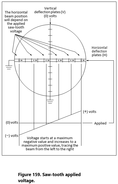
   Vertical Deflection

   If this same signal were applied to the vertical plates, it would also produce a vertical line by causing the beam to trace from the down position to the up position.

   Tracing a Sine Wave

   Reproducing the sine wave on the oscilloscope combines both the vertical and horizontal deflection patterns. [Figure 160] If the sine wave voltage  signal is applied across the vertical deflection plates, the result will be the vertical beam oscillation up and down on the screen. The amount that the beam moves above the centerline will depend on the peak value of the voltage.

   

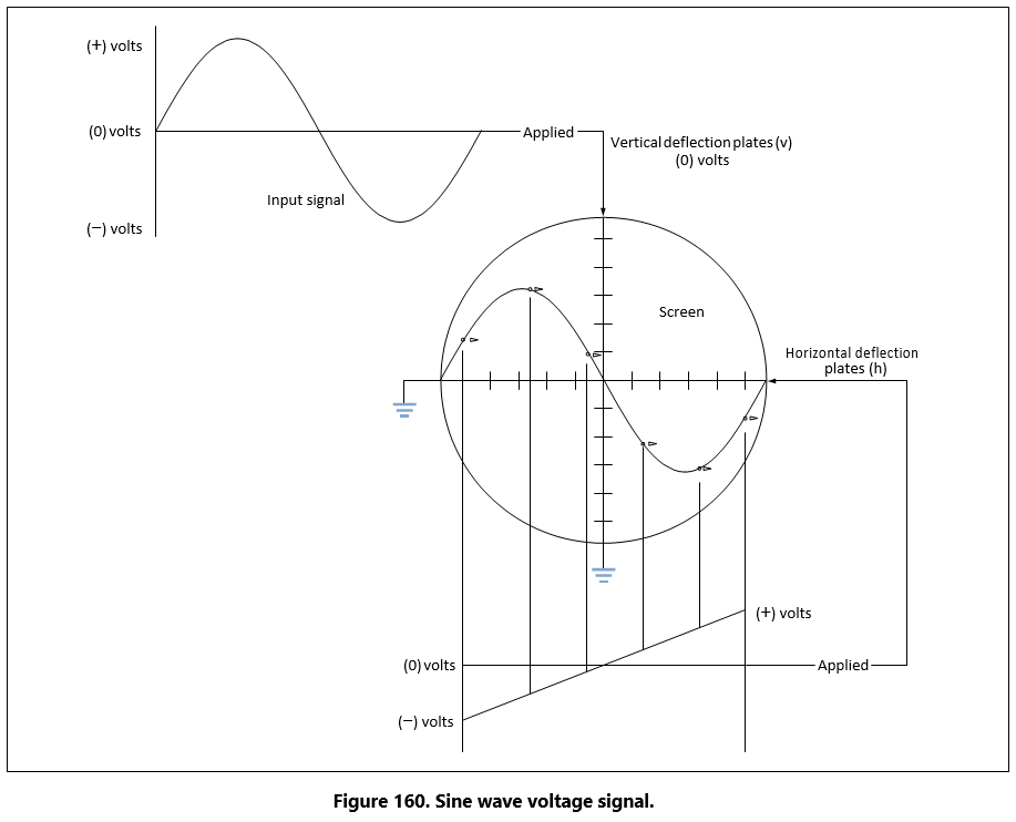
   While the beam is being swept from the left to the right by the horizontal plates, the sine wave voltage is being applied to the vertical plates, causing the form of the input signal to be traced out on the screen.

   Control Features on an Oscilloscope

   While there are many different styles of oscilloscopes, which range from the simple to the complex, they all have some controls in common. Apart from the screen and the ON/OFF switch, some of these controls are listed below.

   Horizontal Position: allows for the adjustment of the neutral horizontal position of the beam. Use this control to reposition the waveform display in order to have a better view of the wave or to take measurements.

   Vertical Position: moves the traced image up or down allowing better observations and measurements.

   Focus: controls the electron beam as it is aimed and converges on the screen. When the beam is in sharp focus, it is narrowed down to a very fine point and does not have a fuzzy appearance.

   Intensity: essentially the brightness of the trace. Controlling the flow of electrons onto the screen varies the intensity. Do not keep the intensity too high for extended testing or when the beam is motionless and forms a dot on the screen. This can damage the screen.

   Seconds/Division: a time-based control, which sets the horizontal sweep rate. Basically, the switch is used to select the time interval that each division on the horizontal scale will represent. These divisions can be seconds, milliseconds or even microseconds. A simple example would be if the technician had the seconds/division control set to 10 μS. If this technician is viewing a waveform that has a period of 4 divisions on the screen, then the period would be 40 μS. The frequency of this waveform can then be determined by taking the inverse of the period. In this case, 1/40 μS will equal a frequency of 25 kHz.

   Volts/Division: used to select the voltage interval that each division on the vertical scale will represent. For example, suppose each vertical division was set to equal 10 mV. If a waveform was measured and had a peak value of 4 divisions, then the peak value in volt- age would be 40 mV.

   Trigger: The trigger control provides synchroniza- tion between the saw-tooth horizontal sweep and the applied signal on the vertical plates. The benefit is that the waveform on the screen appears to be stationary and fixed and not drifting across the screen. A trigger- ing circuit is used to initiate the start of a sweep rather than the fixed saw-tooth sweep rate. In a typical oscil- loscope, this triggering signal comes from the input signal itself at a selected point during the signal’s cycle. The horizontal signal goes through one sweep, retraces back to the left side and waits there until it is triggered again by the input signal to start another sweep.

   Flat Panel Color Displays for Oscilloscopes

   While the standard CRT design of oscilloscope is still in service, the technology of display and control has evolved into use of the flat panel monitors. Further- more, the newer oscilloscopes can even be integrated with the common personal computer (PC). This level of integration offers many diagnostic options unheard of only a few years ago. Some of the features of this technology include easy data capture, data transfer, documentation, and data analysis.

   Digital Multimeter

   Traditionally, the meters that technicians have used have been the analog voltmeter, ammeter, and the ohmmeter. These have usually been combined into the same instrument and called a multimeter or a VOM (volt-ohm-milliammeter). This approach has been both convenient and economical. Digital multimeters (DMM) and digital voltmeters (DVM) have now become more common due to their ease of use. These meters are easier to read and provide greater accuracy when compared to the older analog units with needle movement. The multimeter’s single-coil movement requires a number of scales, which are not always easy to read accurately. In addition, the loading character- istics due to the internal resistance sometimes affect the circuit and the measurements. Not only does the DVM offer greater accuracy and less ambiguity, but also higher input resistance, which has less of a loading effect and influence on a circuit.

   Chapter: 16 Basic Circuit Analysis and Troubleshooting

   Troubleshooting is the systematic process of recognizing the symptoms of a problem, identifying the possible cause, and locating the failed component or conductor in the circuit. To be proficient at troubleshooting, the technician must understand how the circuit operates and know how to properly use the test equipment. There are many ways in which a system can fail and to cover all of the possibilities is beyond the scope of this text. However, there are some basic concepts that will enable the technician to handle many of the common faults encountered in the electronics.

   Before starting a discussion on basic circuits and

   troubleshooting, the following definitions are given.

   • Short circuit — an unintentional low resistance path between two components in a circuit or between a component/conductor and ground. It usually creates high current flow, which will burn out or cause damage to the circuit conductor or components.
   • Open circuit — a circuit that is not a complete or continuous path. An open circuit represents an infinitely large resistance. Switches are common devices used to open and close a circuit. Some- times a circuit will open due to a component fail- ure, such as a light bulb or a burned out
   • Continuity — the state of being continuous, uninterrupted or connected together; the opposite of a circuit that is not broken or does not have an
   • Discontinuity — the opposite of continuity, indicating that a circuit is broken or not

   Voltage Measurement

   Voltage is measured across a component with a voltmeter or the voltmeter position on a multimeter. Usually, there is a DC and anAC selection on the meter. Before the meter is used for measurements, make sure that the meter is selected for the correct type of voltage. When placing the probes across a component to take a measurement, take care to ensure that the polarity is correct. [Figure 161] Standard practice is for the red meter lead to be installed in the positive (+) jack and the black meter lead to be installed in the negative meter j ack (−). Then when placing the probes across or in parallel with a component to measure the voltage, the leads should match the polarity of the component. The red lead shall be on the positive side of the component and the black on the negative side, which will prevent damage to the meter or incorrect readings.

   All meters have some resistance and will shunt some of the current. This has the effect of changing the characteristic of the circuit because of this change in current. This is typically more of a concern with older analog type meters. If there are any questions about the magnitude of the voltage across a component, then the meter should be set to measure on the highest voltage range. This will prevent the meter from “pegging” and possible damage. The range should then be selected to low values until the measured voltage is read at the mid-scale deflection. Readingstaken at mid-scale are the most accurate.

   Current Measurement

   Current is measured with the ammeter connected in the current path by opening or breaking the circuit and inserting the meter in series as shown in Figure 161 Standard practice is for the red meter lead to be installed in the positive (+) jack and the black meter lead to be installed in the negative meter jack (−). The positive side of the meter is connected towards the positive voltage source. Ideally, the meter should not alter the current and influence the circuit and the measurements. However, the meter does have some effect because of its internal resistance that is connected with the rest of the circuit in series. The resistance is rather small and for most practical purposes, this can be neglected.

   

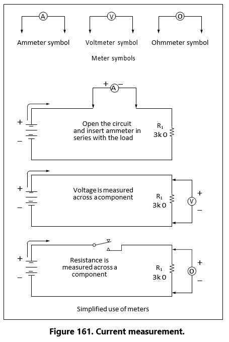
   Checking Resistance in a Circuit

   The ohmmeter is used to measure the resistance. In its more basic form, the ohmmeter consists of a variable resistor in series with a meter movement and a voltage source. The meter must first be adjusted before use.

   Refer to Figure 162 for meter configurations during adjustments. When the meter leads are not connected (open), the needle will point to the full left-hand position, indicating infinite resistance or and open circuit. With the lead placed together, the circuit is shorted as shown with the meter needle to the full right-hand position. When a connection is made, the internal battery is allowed to produce a current through the movement coil, causing a deflection of the needle in proportion to the value of the external resistance. In this case, the resistance is zero because the leads are shorted.

   

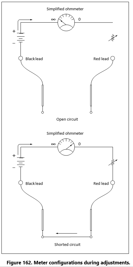
   The purpose of the variable resistor in the meter is to adjust the current so that the pointer will read exactly zero when the leads are shorted. This is needed because as the battery continues to be used, the voltage will change, thus requiring an adjustment. The meter should be “zeroed” before each use.

   To check the value of a resistor, the resistor must be disconnected from the circuit. This will prevent any possible damage to the ohmmeter, and it will prevent the possibility of any inaccurate readings due to the circuit being in parallel with the resistor in question. [Figure 163]

   

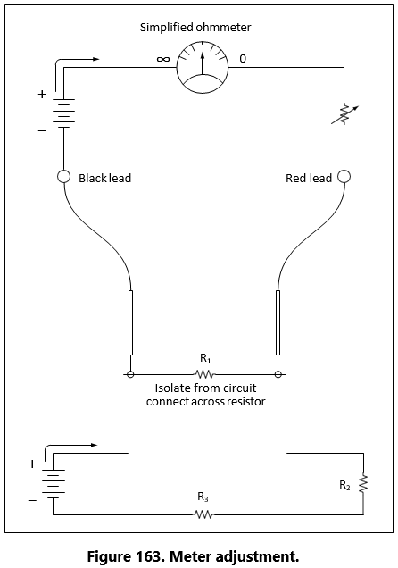
   Continuity Checks

   In many cases, the ohmmeter is not used for measuring the resistance of a component but to simply check the integrity of a connection from one portion of a circuit to another. If there is a good connection, then the ohmmeter will read a near zero resistance or a short. If the circuit is open or has a very poor connection at some point like an over-crimped pin in a connector, then the ohmmeter will read infinity or some very high resistance. Keep in mind that while any measurement is being taken, contact with the circuit or probes should be avoided. Contact can introduce another parallel path and provide misleading indications.

   Capacitance Measurement

   Figure 164 illustrates a basic test of a  capacitor  with an ohmmeter. There are usually two common modes of fail for a capacitor. One is a complete failure characterized by short circuit through the capacitor due to the dielectric breaking down or an open circuit. The more insidious failure occurs due to degradation, which is a gradual deterioration of the capacitor’s characteristics.

   If a problem is suspected, remove the capacitor from the circuit and check with an ohmmeter. The first step is to short the two leads of the capacitor to ensure that it is entirely discharged. Next, connect the two leads as shown in Figure 164 across the capacitor and observe the needle movement. At first, the needle should indicate a short circuit. Then as the capacitor begins to charge, the needle should move to the left or infinity and eventually indicate an open circuit. The capacitor takes its charge from the internal battery of the ohmmeter. The greater the capacitance, the longer it will take to charge. If the capacitor is shorted, then the needle will remain at a very low or shorted resistance. If there is some internal deterioration of the dielectric, then the needle will never reach a high resistance but some intermediate value, indicating a current.

   

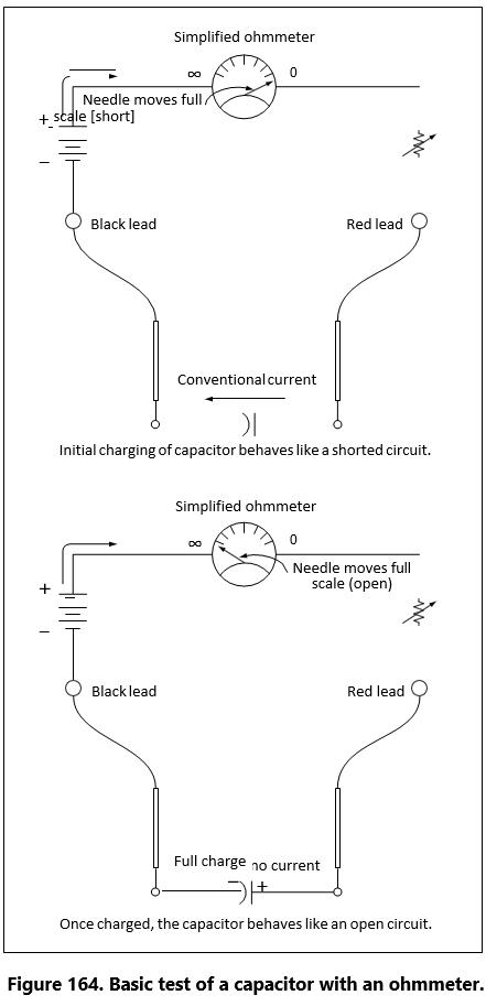
   Inductance Measurement

   The common mode of failure in an inductor is an open. To check the integrity of an inductor, it must be removed from the circuit and tested as an isolated component just like the capacitor. If there is an open in the inductor, a simple check with an ohmmeter will show it as an open circuit with infinite resistance. If in fact the inductor is in good condition, then the ohm- meter will indicate the resistance of the coil.

   On occasions, the inductor will fail due to overheating. When the inductor is overheated, it is possible for the insulation covering the wire in the coil to melt, causing a short. The effects of a shorted coil are that of reduc- ing the number of turns. At this point, further testing of the inductor must be done with test equipment not covered in this text.

   Troubleshooting the Open Faults in Series Circuit One of the most common modes of failure is the “open” circuit. A component, such as a resistor, can overheat

   due to the power rating being exceeded. Other more

   frustrating problems can happen when a “cold” solder joint cracks leaving a wire disconnected from a relay or connector. This type of damage can occur during routine maintenance after a technician has accessed an area for inspections. In many cases, there is no visual indication that a failure has occurred, and the soon-to-be-frustrated technician is unaware  that there is a problem until power is reapplied to the electronics for scheduled operations.

   The first example is a simplified diagram shown in Figures 165 through 167. The circuit depicted in Figure 165 is designed to cause current to flow through a lamp, but because of the open resistor, the lamp will not light. To locate this open, a voltmeter or an ohmmeter should be used.

   

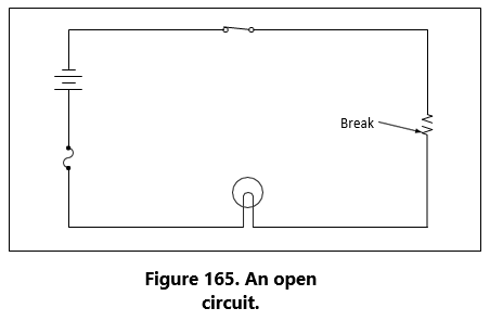
   Tracing Opens with the Voltmeter

   A general procedure to follow in this case is to measure the voltage drop across each component in the circuit, keeping in mind the following points. If there is an open in a series circuit, then the voltage drops on sides of the component. In this case, the total voltage must appear across the open resistor as per Kirchhoff’s voltage law.

   If a voltmeter is connected across the lamp, as shown in Figure 166, the voltmeter will read zero. Since no current can flow in the circuit because of the open resistor, there is no voltage drop across the lamp indi-cating that the lamp is good.

   

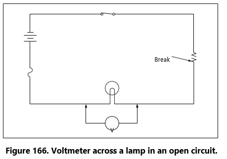
   Next, the voltmeter is connected across the open resis- tor, as shown in Figure 167. The voltmeter has  closed the circuit by shunting (paralleling) the burned out resistor, allowing current to flow. Current will flow from the negative terminal of the battery, through the switch, through the voltmeter and the lamp, back to the positive terminal of the battery. However, the resistance of the voltmeter is so high that only a very small current flows in the circuit. The current is too small to light the lamp, but the voltmeter will read the battery voltage.

   

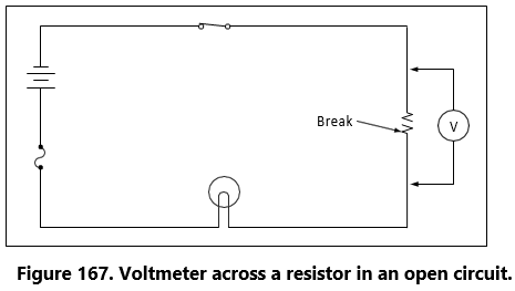
   Tracing Opens with the Ohmmeter

   A simplified circuit as shown in Figures 168 and 169 illustrates how to locate an open in a series circuit using the ohmmeter. A general rule to keep in mind when troubleshooting with an ohmmeter is: when an ohmmeter is properly connected across a circuit component and a resistance reading is obtained, the component has continuity and is not open.

   When an ohmmeter is used, the circuit component   to be tested must be isolated and the power source removed from the circuit. In this case, as shown in Figure 168, these requirements can be met by opening the circuit switch. The ohmmeter is zeroed and across all good components will be zero. The voltage drop across the open component will equal the total voltage across the series combination. This condition happens because the open component will prevent current to pass through the series circuit. With there being no current, there can be no voltage drop across any of the good components. Because the current is zero, it can be determined by Ohm’s law that E = IR = 0 volts across a component. The voltage is the same on both places across (in parallel with) the lamp. In this testing configuration, some value of resistance is read indicating that the lamp is in good condition and is not the source of the open in the circuit.

   

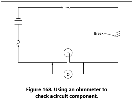
   Now the technician should move to the resistor and place the ohmmeter probe across it as shown in Figure 169. When the  ohmmeter  is  connected across the open resistor, it indicates infinite resistance, or a discontinuity. Thus, the circuit open has now been located.

   

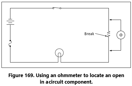
   Troubleshooting the Shorting Faults in Series Circuit

   An open fault can cause a component or system not to work, which can be critical and hazardous. A shorting fault can potentially be more of a severe nature than the open type of fault. A short circuit, or “short,” will cause the opposite effect. A short across a series circuit produces a greater than normal current flow. Faults of this type can develop slowly when a wire bundle is not properly secured and is allowed to chafe against the airframe structure or other systems such as hydraulic lines. Shorts can also occur due to a careless technician using incorrect hardware when installing an interior. If screws that are too long are used to install trim, it is possible to penetrate a wire bundle immediately causing numerous shorts. Worse yet, are the shorts that are not immediately seen but “latent” and do not show symptoms until the electronics is in service. Another point to keep in mind is when closing panels. Wires can become pinched between the panel and the airframe causing either a short or a latent, intermittent short. The simplified circuit, shown in Figures 170 through 172, and Figure 173 will be used to illustrate troubleshooting a short in a series circuit.

   In Figure 170, a circuit is designed to light a lamp. A resistor is connected in the circuit to limit current flow. If the resistor is shorted, as shown in the illustration, the current flow will increase and the lamp will become brighter. If the applied voltage were high enough, the lamp would burn out, but in this case the fuse would protect the lamp by opening first.

   

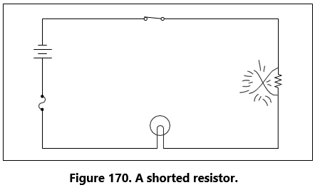
   Usually a short circuit will produce an open circuit by either blowing (opening) the fuse or burning out a circuit component. But in some circuits, such as that illustrated in Figure 171, there may be additional resistors which will not allow one shorted resistor to increase the current flow enough to blow the fuse or burn out a component. Thus, with one resistor shorted out, the circuit will still function since the power dis- sipated by the other resistors does not exceed the rating of the fuse.

   

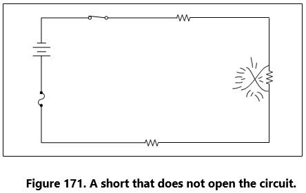
   Tracing Shorts with the Ohmmeter

   The shorted resistor shown in Figure 172 can be located with an ohmmeter. First the switch is opened to isolate the circuit components. In Figure 172, this circuit is shown with an ohmmeter connected across each of the resistors. Only the ohmmeter connected across the shorted resistor shows a zero reading, indi- cating that this resistor is shorted.

   

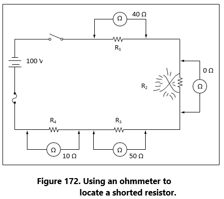
   Tracing Shorts with the Voltmeter

   To locate the shorted resistor while the circuit is functioning, a voltmeter can be used. Figure 173 illustrates that when a voltmeter is connected across any of the resistors, which are not shorted, a portion of the applied voltage will be indicated on the voltmeter scale. When it is connected across the shorted resistor, the voltmeter will read zero.

   

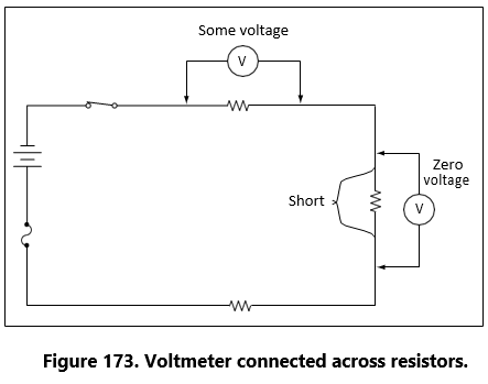
   Troubleshooting the Open Faults in Parallel Circuit

   The procedures used in troubleshooting a parallel circuit are sometimes different from those used in a series circuit. Unlike a series circuit, a parallel cir- cuit has more than one path in which current flows. A voltmeter cannot be used, since, when it is placed across an open resistor, it will read the voltage drop in a parallel branch. But an ammeter or the modified use of an ohmmeter can be employed to detect an open branch in a parallel circuit.

   If the open resistor shown in Figure 174 was not visually apparent, the circuit might appear to be functioning properly, because current would continue to flow in the other two branches of the circuit. To determine that the circuit is not operating properly,  a determination must be made as to how the circuit should behave when working properly. First, the total resistance, total current, and the branch currents of the circuit should be calculated as if there were no open in the circuit. In this case, the total resistance can be simply determined by:

   

   

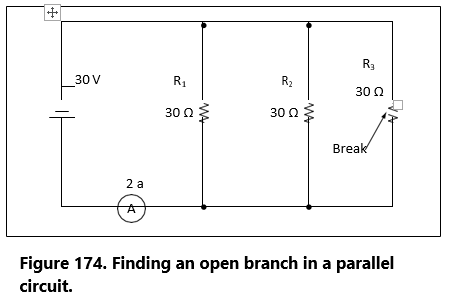
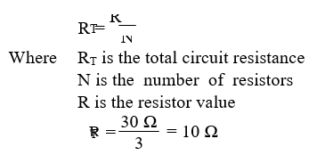
   The total current of the circuit can now be determined by using Ohm’s law:

   

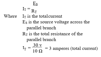
   Each branch current should be determined in a similar manner. For the first branch, the current is:

   

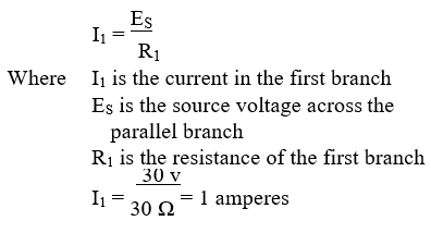
   Because the other two branches are of the same resistive value, then the current in each of those branches will be 1 ampere also. Adding up the amperes in each branch confirms the initial calculation of total current being 3 amperes.

   Tracing an Open with an Ammeter

   If the technician now places an ammeter in the circuit, the total current would be indicated as 2 amperes as show in Figure 174 instead of the calculated 3 amperes. Since 1 ampere of current should be flowing through each branch, it is obvious that one branch is open. If the ammeter is then connected into the branches, one after another, the open branch will eventually be located by a zero ammeter reading.

   Tracing an Open with an Ohmmeter

   A modified use of the ohmmeter can also locate this type of open. If the ohmmeter is connected across the open resistor, as shown in Figure 175, an erroneous reading of continuity would be obtained. Even though the circuit switch is open, the open resistor is still in parallel with R1 and R2, and the ohmmeter would indicate the open resistor had a resistance of 15 ohms, the equivalent resistance of the parallel combination of R1 and R2.

   

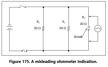
   Therefore, it is necessary to open the circuit as shown in Figure 176 in order to check the resistance of R3. In this way, the resistor is not shunted (paralleled) by R1 and R2. The reading on the ohmmeter will now indicate infinite resistance, which means the open component has been isolated.

   

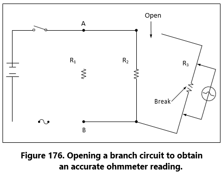
   Troubleshooting the Shorting Faults in Parallel Circuit

   As in a series circuit, a short in a parallel circuit will usually cause an open circuit by blowing the fuse. But, unlike a series circuit, one shorted component in a parallel circuit will stop current flow by causing the fuse to open. Refer to the circuit in Figure 177. If resistor R3 is shorted, a path of almost zero resistance will be offered the current, and all the circuit current will flow through the branch containing the shorted resistor. Since this is practically the same as connecting a wire between the terminals of the battery, the current will rise to an excessive value, and the fuse will open. Since the fuse opens almost as soon as a resistor shorts out, there is no time to perform a current or voltage check. Thus, troubleshooting a parallel DC circuit for a shorted component should be accomplished with an ohmmeter. But, as in the case of checking for an open resistor in a parallel circuit, a shorted resistor can be detected with an ohmmeter only if one end of the shorted resistor is disconnected and isolated from the rest of the circuit.

   

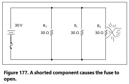
   Troubleshooting the Shorting Faults in Series-Parallel Circuit

   Logic in Tracing an Open

   Troubleshooting a series-parallel resistive circuit involves locating malfunctions similar to  those found in a series or a parallel circuit. Figures 178 through 180 illustrate three points of failure in a series-parallel circuit and their generalized effects.

   1. In the circuit shown in Figure 178, an open has occurred in the series portion of the circuit. When the open occurs anywhere in the series portion of a series-parallel circuit, current flow in the entire circuit will stop. In this case, the circuit will not function, and the lamp, L1, will not be lit.
      
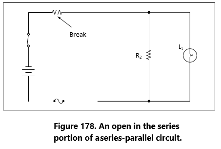
   2. If the open occurs in the parallel portion of a series-parallel circuit, as shown in Figure 179, part of the circuit will continue to function. In this case, the lamp will continue to burn, but its brightness will diminish, since the total resistance of the circuit has increased and the total current has decreased.
      
   3. If the open occurs in the branch containing the lamp, as shown in Figure 180, the circuit will continue to function with increased resistance and decreased current, but the lamp will not light.

   

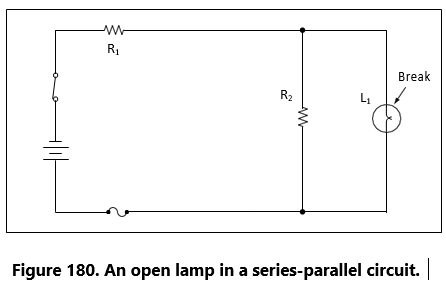
   Tracing Opens with the Voltmeter

   To explain how the voltmeter and ohmmeter can be used to troubleshoot series-parallel circuits, the circuit shown in Figure 181 has been labeled at various points. A point-to-point  description  is  listed below with expected results:
   

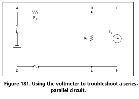
   1. By connecting a voltmeter between points A and D, the battery and switch can be checked for
   2. By connecting the voltmeter between points A and B, the voltage drop across R1 can be This voltage drop is a portion of the applied voltage.
   3. If R1 is open, the reading between B and D will be zero.
   4. By connecting a voltmeter between A and E, the continuity of the conductor between the positive terminal of the battery and point E, as well as the fuse, can be checked. If the conductor or fuse is open, the voltmeter will read zero.
   5. If the lamp is burning, it is obvious that no open exists in the branch containing the lamp, and the voltmeter could be used to detect an open in the branch containing R2 by removing lamp, L1, from the circuit.

   Troubleshooting the series portion of a series-parallel circuit presents no difficulties, but in the parallel portion of the circuit, misleading readings can be obtained.