Forecasting Solar Radiation and Photovoltaic Power Help

Overview of Solar Radiation Resource Concepts

1.1 Introduction

This chapter discusses standard terms that are used to illustrate the key characteristics of solar radiation—the fuel for all solar technologies.

Beginning with the Sun as the source, this chapter presents an overview of the effects of Earth’s orbit and atmosphere on the possible types and magnitudes of solar radiation available for energy conversion. This overview concludes with an important discussion of the estimated uncertainties associated with solar resource data as affected by the experimental and modeling methods used to produce the data.

1.2 Radiometric Terminology

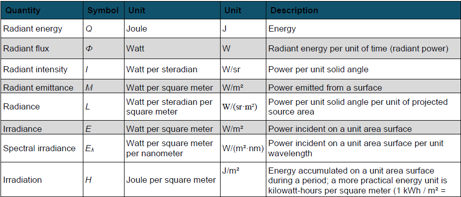
Before discussing solar radiation further, it is important to understand basic radiometric terms. Radiant energy, flux, power, and other concepts used in this course are summarized in Table 1-1.

Table 1-1. Radiometric Terminology and Units

1.3 Extraterrestrial Irradiance

Any object with a temperature above absolute zero Kelvin emits radiation. With an effective surface temperature of ≈5800 K, the Sun behaves like a quasi-static blackbody and emits radiation over a wide range of wavelengths, with a distribution that is close to that predicted by Planck’s law (Figure 1-1). This constitutes the solar spectral power distribution, or solar spectrum. For terrestrial applications, the useful solar spectrum, also called the shortwave spectrum (≈290–4000 nm), includes the spectral regions called ultraviolet (UV), visible, and near-infrared (NIR) (Figure 1-1). The latter is the part of the infrared spectrum that is below 4000 nm in the solar spectrum. In contrast, the longwave (or far-infrared) spectrum extends beyond 4 μm, where the planetary thermal emission is dominant. Based on a recent determination (Gueymard 2018a), most spectral irradiance (98.5%) of the extraterrestrial spectrum (ETS), is contained in the wavelength range from 290–4000 nm. In what follows, broadband solar radiation will always refer to this spectral range, unless specified otherwise.

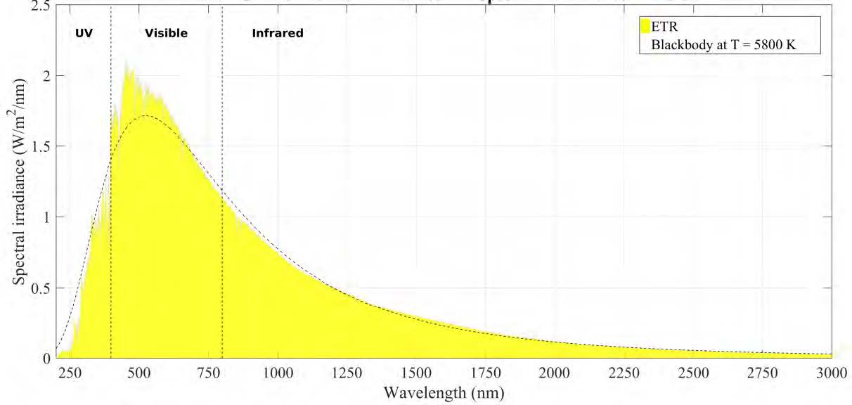
Various ETS distributions have been derived based on ground measurements, extraterrestrial measurements, and physical models of the Sun’s output. Some historical perspective is offered by Gueymard (2004, 2006, 2018a). All distributions contain some deviations from the current standard extraterrestrial spectra used by ASTM Standard E490 (2019) (Figure 1-1). A new generation of ETS distribution, based on recent spectral measurements from space, was recently published (Gueymard 2018a).

1.4 Solar Constant and Total Solar Irradiance

The total radiant power from the Sun is nearly constant. The solar output (radiant emittance) is called the total solar irradiance (TSI) and can be obtained as the integration of the ETS at 1 AU (astronomical unit, approximate average Sun-Earth distance) over all wavelengths. TSI was commonly called the solar constant (SC) until slight temporal variations were discovered (Fröhlich and Lean 1998, 2004; Kopp and Lean 2011). The solar constant is now defined as the long-term mean TSI. Both TSI and solar constant are made independent from the actual Sun-Earth distance by evaluating them at 1 AU. Small but measurable changes in the Sun’s output and TSI are related to its magnetic activity. There are cycles of approximately 11 years in solar activity, which are accompanied by a varying number of sunspots (cool, dark areas on the Sun) and faculae (hot, bright spots). TSI increases during high-activity periods because the numerous faculae more than counterbalance the effect of sunspots. From an engineering perspective, these TSI variations are relatively small, so the solar constant concept is still useful and perfectly appropriate in solar applications.

Figure 2-2 shows the latest version of a composite TSI time series based on multiple spaceborne instruments that have monitored TSI since 1978 using a variety of instruments and absolute scales (Gueymard 2018b). Estimates are also used for the period from 1976–1978 to make this time series start at the onset of solar cycle 21. The solar cycle numbers are indicated for further reference. (Solar cycle 25 is assumed to have started at the end of 2019, but this is still debated as of this writing.) Figure 2-2 shows the solar constant (always evaluated at 1 AU) as a horizontal solid line.

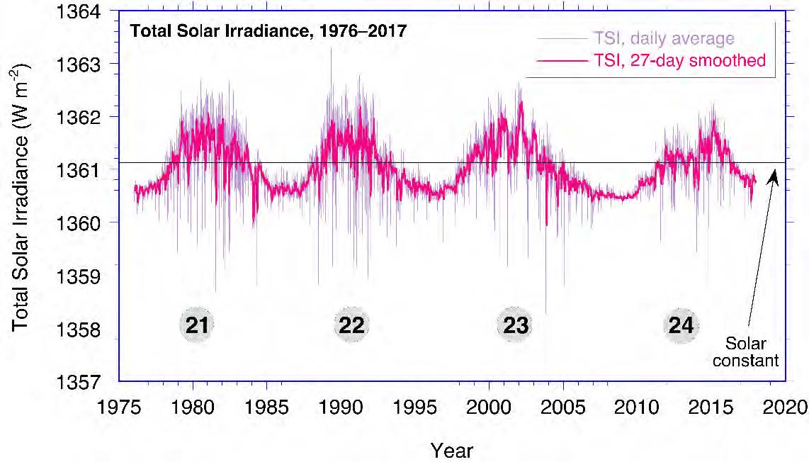
On a daily basis, the passage of large sunspots results in much lower TSI values than the solar constant. The measured variation in TSI resulting from the sunspot cycle is at most ±0.2%, only twice the precision (i.e., repeatability—not total absolute accuracy, which is approximately ±0.5%) of the most accurate radiometers measuring TSI in space. There is, however, some large variability in a few spectral regions—especially the UV (wavelengths less than 400 nm)—caused by solar activity.

Historic determinations of solar constant have fluctuated throughout time (Gueymard 2006; Kopp 2016). At the onset of the 21st century, it was 1366.1 ± 7 W/m2 (ASTM 2000; Gueymard 2004). More recent satellite observations using advanced sensors and better calibration methods, however, have shown that the solar constant is somewhat lower: ≈1361 W/m2. After careful reexamination and corrections of decades of past satellite-based records, Gueymard (2018b) proposed a revised value of 1361.1 W/m2.

According to astronomical computations such as those made by the National Renewable Energy Laboratory’s (NREL’s) solar position software (https://midcdmz.nrel.gov/spa/), using SC ≈1361 W/m2, the seasonal variation of ±1.7% in the Sun-Earth distance causes the irradiance at the top of the Earth’s atmosphere to vary from ≈1409 W/m2 (+3.5%) near January 3 to ≈1315 W/m2 (–3.3%) near July 4. This seasonal variation is systematic and deterministic; hence, it does not include the daily (somewhat random) or cyclical variability in TSI induced by solar activity, which was discussed previously. This variability is normally less than ±0.2% and is simply ignored in the practice of solar resource assessments.

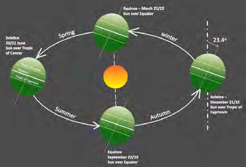
1.5 Solar Geometry

The amount of radiation exchanged between two objects is affected by their separation distance. The Earth’s elliptical orbit (eccentricity 0.0167) brings it closest to the Sun in January and farthest from the Sun in July, as mentioned. The average Sun-Earth distance is close to the new definition of the AU, which is exactly 149,597,870,700 m, as introduced in 2012 by the International Astronomical Union and recognized as a Système International (SI) unit in 2014 by the International Bureau of Weights and Measures (BIPM). Figure 2-3 shows the Earth’s orbit in relation to the northern hemisphere’s seasons, caused by the average ≈23.4° tilt of the Earth’s rotational axis with respect to the plane of the orbit. The solar irradiance available at the top of atmosphere (TOA) is called the extraterrestrial radiation (ETR). ETR (see Eq. 1-1) is the power per unit area, or flux density, in Watts per square meter (W/m2), radiated from the Sun and available at the TOA. Just like ETS, ETR varies with the Sun-Earth distance (r) and annual mean distance (r0):

As indicated in Section 1.4, it is customary to neglect temporal variations in TSI so that TSI can be replaced by the solar constant in Eq. (1-1) for simplification. The Sun-Earth distance correction factor, (r0/r)2, in Eq. 1-1 is normally obtained from sun position algorithms, such as those described in Section 1.6.1. Daily values of sufficient accuracy for most applications can also be found in tabulated form—e.g., Iqbal (2012).

From the TOA, the sun appears as a very bright disk with an angular diameter of ≈0.5° (the actual apparent diameter varies by a small amount, ±1.7%, because the Sun-Earth distance varies) surrounded by a completely black sky, apart from the light coming from stars and planets. This angle can be determined from the distance between the Earth and the Sun and the latter’s apparent diameter. More precisely, a point at the top of the Earth’s atmosphere intercepts a cone of light from the hemisphere of the Sun facing the Earth with a total angle of 0.53°±1.7% at the apex and a divergence angle from the center of the disk of 0.266° (half the apex angle, yearly average). Because the divergence angle is very small, the rays of light emitted by the Sun are nearly parallel; these are called the solar beam. The interaction of the solar beam with the terrestrial atmosphere is discussed next.

1.6 Solar Radiation and the Earth’s Atmosphere

The Earth’s atmosphere can be seen as a continuously variable filter for the solar ETR as it reaches the surface. Figure 1-4 illustrates the “typical” absorption of solar radiation by atmospheric constituents such as ozone, oxygen, water vapor, or carbon dioxide. The amount of atmosphere the solar photons must traverse, also called the atmospheric path length or air mass (AM), depends on the relative position of the observer with respect to the sun’s position in the sky (Figure 1-4). By convention, air mass one (AM1) is defined as the amount of atmospheric path length observed when the sun is directly overhead. As a first approximation, and for low zenith angles, air mass is geometrically related to the solar zenith angle (SZA). Actually, air mass is approximately equal to the secant of SZA, or 1/cos(SZA). Air mass 1.5 (AM1.5) is a key quantity in solar applications and corresponds to SZA = 48.236° (Gueymard, Myers, and Emery, 2002). Air mass two (AM2) occurs when SZA is ≈60° and has twice the path length of AM1. By extrapolation, one refers to the value at the TOA as AM0 (Myers 2013).

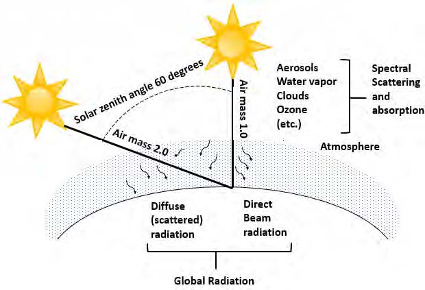
The cloudless atmosphere contains gaseous molecules and particulates (e.g., dust and other aerosols) that reduce the ETR as it progresses farther down through the atmosphere. This reduction is caused mostly by scattering (a change of a photon’s direction of propagation) and also by absorption (a capture of radiation). Finally, clouds are the major elements that modify the ETR (also by scattering and absorption) on its way to the surface or to a solar collector.

Absorption converts part of the incoming solar radiation into heat and raises the temperature of the absorbing medium. Scattering redistributes the radiation in the hemisphere of the sky dome above the observer, including reflecting part of the radiation back into space. The longer the path length through the atmosphere, the more radiation is absorbed and scattered. The probability of scattering—and hence of geometric and spatial redistribution of the solar radiation—increases as the path (air mass) from the TOA to the ground increases.

Part of the radiation that reaches the Earth’s surface is eventually reflected back into the atmosphere. A fraction of this returns to the surface through a process known as backscattering. The actual geometry and flux density of the reflected and scattered radiation depend on the reflectivity and physical properties of the surface and constituents in the atmosphere, especially clouds and aerosols.

Based on these interactions between the radiation and the atmosphere, the terrestrial solar radiation is divided into two components: direct beam radiation, which refers to solar photons that reach the surface without being scattered or absorbed, and diffuse radiation, which refers to photons that reach the observer after one or more scattering events with atmospheric constituents. These definitions and their usage for solar energy are discussed in detail in Section 1.7.

Ongoing research continues to increase our understanding of the properties of atmospheric constituents, ways to estimate them, and their impact on the magnitude of solar radiation in the atmosphere at various atmospheric levels and at the surface. This is of great importance to those who measure and model solar radiation fluxes.

1.6.1 Relative Motions of the Earth and Sun

The amount of solar radiation available at the TOA is a function of TSI and the Sun-Earth distance at the time of interest, per Eq. (1-1). The slightly elliptical orbit of the Earth around the Sun was briefly described in Section 1.5 and is shown in Figure 1-3. The Earth rotates around an axis through the geographic north and south poles, inclined at an average angle of ≈23.4° to the plane of the Earth’s orbit. The axial tilt of the Earth’s rotation also results in daily variations in the solar geometry during any year.

In the Northern Hemisphere, at latitudes above the Tropic of Cancer (23.437° N) near midday, the sun is low on the horizon during winter and high in the sky during summer. Summer days are longer than winter days because of progressive changes where the sun rises and sets. Similar transitions take place in the Southern Hemisphere. All these changes result in changing geometry of the solar position in the sky with respect to time of year and specific location. Similarly, the resulting yearly variation in the solar input creates seasonal variations in climate and weather at each location. The solar position in the sky corresponds to topocentric angles, as follows:

• The solar elevation angle is defined as the angle formed by the direction of the sun and the local horizon. It is the complement of SZA, i.e., 90°–SZA.
• The solar azimuth angle is defined as the angle formed by the projection of the direction of the sun on the horizontal plane defined eastward from true north, following the International Organization for Standardization (ISO) 19115 standard. For example, 0° or360° = due north, 90° = due east, 180° = due south, and 270° = due west.

An example of apparent sun path variations for various periods of the year is depicted in Figure 1-5. Because of their significance in performing any analysis of solar radiation data or any radiation model calculation, the use of solar position calculations of sufficient accuracy is necessary, such as those derived from NREL’s Solar Position Algorithm4 (Reda and Andreas2003, 2004). This algorithm predicts solar zenith and azimuth angles as well as other related parameters such as the Sun-Earth distance and the solar declination. All this is possible in the period from 2000 B.C. to 6000 A.D. with an SZA standard deviation of only ≈0.0003° (1”). To achieve such accuracy during a long period, this algorithm is very time consuming, with approximately 2300 floating operations and more than 300 direct and inverse trigonometric functions at each time step. Other algorithms exist, differing in the attained accuracy and in their period of validity. Various strategies exist to reduce operations, such as reducing the period of validity while maintaining high accuracy (Blanc and Wald 2012; Grena 2008; Blanco-Muriel etal. 2001) or keeping a long period while reducing the accuracy (Michalsky 1988).

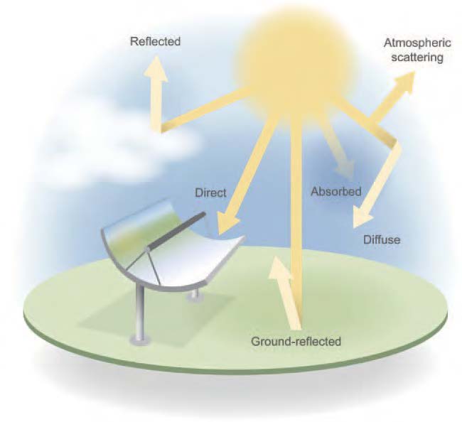
1.7 Solar Resource and Components Radiation can be transmitted, absorbed, or scattered in varying amounts by an attenuating medium, depending on wavelength. Complex interactions of the Earth’s atmosphere with solar radiation result in three fundamental broadband components of interest to solar energy conversion technologies:

• Direct normal irradiance (DNI): solar (beam) radiation from the sun’s disk itself—of interest to concentrating solar technologies (CST), tracked collectors, and other solar technologies because of incidence angle dependent efficiency
• Diffuse horizontal irradiance (DHI): scattered solar radiation from the sky dome(excluding the sun and thus DNI)5
• Global horizontal irradiance (GHI): geometric sum of the direct and diffuse horizontalcomponents (also called the total hemispheric irradiance)
• Global tilted irradiance (GTI): geometric sum of the direct, sky diffuse, and ground-reflected components on a tilted surface. GTI is also referred to as the plane-of-array(POA) irradiance in the photovoltaic (PV) literature.
• Global normal irradiance (GNI): geometric sum of the direct, sky diffuse, and ground-reflected components on a tracking surface that remains perpendicular to the sunbeam.

The radiation components are shown in Figure 1.6.

These basic solar components are related to SZA by the fundamental expression:

where AI is the angle of incidence of the solar beam onto the tilted surface, SVF is the sky view factor between the collector and the visible part of the sky, GVF is the ground view factor between the collector and the visible part of the foreground surface, and RHI is the global reflected horizontal irradiance.

1.7.1 Direct Normal Irradiance and Circumsolar Irradiance

By definition, DNI is the irradiance on a surface perpendicular to the vector (i.e., normal incidence) from the observer to the center of the sun caused by radiation that was not scattered by the atmosphere out of the region appearing as the solar disk (WMO 2018). This strict definition is useful for atmospheric physics and radiative transfer models, but it results in a complication for ground observations: it is not possible to measure whether or not a photon was scattered if it reaches the observer from the direction in which the solar disk is seen. Therefore, DNI is usually interpreted in a less stringent way in the world of solar energy. Direct solar radiation is understood as the “radiation received from a small solid angle centered on the sun’s disk” (ISO 2018). The size of this “small solid angle” for DNI measurements is recommended to be 5 ∙ 10-3 sr (corresponding to ≈2.5° half angle) (WMO 2018). This recommendation is approximately 10 times larger than the angular radius of the solar disk itself based on no-atmosphere geometry, whose yearly average is 0.266°, as mentioned earlier. This relaxed definition is necessary for practical reasons because the instruments used for DNI measurement (pyrheliometers) need to track or follow the sun throughout its path of motion in the sky, and small tracking errors are to be expected. The relatively large field of view (FOV) of pyrheliometers reduces the effect of such tracking errors. Similarly, DHI must be obtained by masking the sun from the pyranometer detector with a small shade. An FOV with a radius of 2.5° is necessary to avoid the impact of tracking errors (e.g., wind-induced tracking errors) and to maintain an FOV complementary to that of the pyrheliometer.

To understand the definition of DNI and how it is measured by pyrheliometers in practice, the role of circumsolar radiation—scattered radiation coming from the annulus surrounding the solar disk—must be discussed. (The reader is referred to the detailed review, based on both experimental and modeling results, found in Blanc et al. (2014).) Because of forward scattering of direct sunlight in the atmosphere, the circumsolar region closely surrounding the solar disk (solar aureole) looks very bright and can alter the observed sunshape (Buie et al. 2003). The sunshape—a quantity not to be confused with the “shape of the Sun”—is the azimuthally averaged radiance profile as a function of the angular distance from the center of the sun normalized to 1 at the apparent sun’s disc center. The radiation coming from this region is called the circumsolar radiation. For the typical FOV of modern pyrheliometers (2.5°), circumsolar radiation contributes a variable amount, depending on atmospheric conditions, to the DNI measurement. Determining the magnitude of the circumsolar radiation is of interest in CST applications because DNI measurements are typically larger than the beam irradiance that can be used in concentrating systems. This causes an overestimate of CST plant production because the FOV of the concentrators (typically of the order of 1° or even less) is much smaller than the FOV of the pyrheliometers that are used on-site to determine the incident DNI.

The circumsolar contribution to the observed DNI can be quantified if the radiance distribution within the circumsolar region and the so-called penumbra function of the pyrheliometer are known. The latter is a characteristic of the instrument and can be derived from the manufacturer’s data. The former, however, is difficult to determine experimentally with current instrumentation. For instance, a method based on two commercial instruments (a sun and aureole measurement system and a sun photometer) has been presented (Gueymard 2010; Wilbert et al. 2013). Other instruments that can measure the circumsolar irradiance are documented in Wilbert et al. (2012, 2018), Kalapatapu et al. (2012), and Wilbert (2014).

To avoid additional measurements, substantial modeling effort is required and might involve estimation of the spectral distribution (Gueymard 2001). Some specific input data are rarely accessible in real time, particularly when a thin ice cloud (cirrus) reduces DNI but considerably increases the circumsolar contribution. Despite these difficulties and because of the special needs of the solar industry, new specialized radiative models have been developed recently to evaluate the difference between the true and apparent DNI using various types of observations (Eissa et al. 2018; Räisänen and Lindfors 2019; Sun et al. 2020; Xie et al. 2020). More research is being conducted to facilitate the determination of the circumsolar fraction at any location and any instant as part of solar resource assessments.

1.7.2 Diffuse Irradiance

A cloudless atmosphere absorbs and scatters some radiation out of the direct beam before it reaches the Earth’s surface. Scattering occurs in essentially all directions, away from the specific path of the incident beam radiation. This scattered radiation constitutes the sky diffuse radiation in the hemisphere above the surface. In particular, the Rayleigh scattering theory explains why the sky appears blue (short wavelengths, in the blue and violet parts of the spectrum, are scattered more efficiently by atmospheric molecules) and why the sun’s disk appears yellow-red at sunrise and sunset (blue wavelengths are mostly scattered out of the direct beam, whereas the longer red wavelengths undergo less scattering, resulting in a red shift). As mentioned above, the sky radiation in the hemisphere above the local surface is referred to as DHI. A more technical and practical definition of DHI is that it represents all radiation from the sky dome except what is considered DNI; hence, in practice, DHI is the total diffuse irradiance from the whole-sky hemisphere minus the 2.5° annulus around the sun center.

DHI includes radiation scattered by molecules (Rayleigh effect), aerosols (Mie effect), and clouds (if present). It also includes the backscattered radiation that is first reflected by the surface and then re-reflected downward by the atmosphere or clouds. The impact of clouds is difficult to model because they have optical properties that can vary rapidly over time and can also vary considerably over the sky hemisphere. Whereas a single and homogenous cloud layer can be modeled with good accuracy, complex three-dimensional cloud scenes present extreme challenges (Hogan and Shonk 2012).

1.7.3 Global Irradiance

The total hemispherical solar radiation on a horizontal surface, or GHI, is the sum of DHI and the projected DNI to the horizontal surface, as expressed by Eq. 1-2. This fundamental equation is used for data quality assessments, some solar radiation measurement system designs, and atmospheric radiative transfer models addressing the needs for solar resource data. Because GHI is easier—and less expensive—to measure than DNI or DHI, most radiometric stations in the world provide only GHI data. It is then necessary to estimate DNI and DHI by using an appropriate separation model, as discussed in the next section.

1.7.4 Solar Resources for Solar Energy Conversion

Obtaining data time series or temporal averages of the solar radiation components—most importantly, GHI and DNI—that relate to a conversion system is the first step in selecting the site-appropriate technology and evaluating the simulated performance of specific system designs. Systems with highly concentrating optics rely solely on DNI. Low-concentration systems might also be able to use some sky diffuse radiation. Flat-plate collectors, fixed or tracking, can use all downwelling radiation components as well as radiation reflected from the ground if in the collector’s FOV.

Solar radiation data are required at all stages of a solar project. Before construction, long time series of historical data are necessary to quantify the solar resource and its variability. During operation, real-time data are typically necessary to verify the performance of the system and to detect problems. In both cases, the required data can be obtained from measurements, modeling, or a combination of both. Typically, measurements are not used exclusively for the early stages of development because (1) long time series of measured irradiance data generally do not exist at the location of interest; (2) measured data, when available, most likely contain gaps that must be filled by modeling; and (3) conducting quality measurements is considerably more costly than operating models (assuming, of course, that the otherwise prohibitively high costs of satellite operations and data management are borne by other agencies). High-quality measurements remain essential, however, because their uncertainty is normally significantly less than that of modeled data , and thus they can serve to validate models and even improve the quality of long-term modeled time series through a “site adaptation” process. The development and validation of solar radiation models is an intricate procedure that requires irradiance observations obtained with very low measurement uncertainty, typically obtained only at research-class stations.

GHI is measured at a relatively large number of stations in the world; however, the quality of such data remains to be verified at most of these stations. Assuming that good-quality GHI data are available at a station of interest, how can the analyst derive the two other components—DNI and DHI—for example, to compute global irradiance on a tilted plane?

There are two possible solutions to this frequent situation. The first is to temporarily ignore the existing GHI data and obtain time series of GHI, DNI, and DHI from a reputable source of satellite-derived data. The modeled and measured GHI data can then be compared for quality assurance and possible bias corrections to the modeled data or, conversely, to determine the quality of the measured data. Both measured and modeled GHI values can incorporate systematic biases. Understanding the magnitude and nature of these biases and how they can affect the calculation is important when determining the uncertainty in the results.

The second method for determining DNI and DHI from GHI data consists of using one of numerous “separation” or “decomposition” models, about which considerable literature exists. Gueymard and Ruiz-Arias (2016) reviewed 140 such models and quantified their performance at 54 high-quality radiometric stations over all continents using data with high temporal resolution (1 minute, in most cases). Previous evaluations had targeted a limited number of models, exclusively using the more conventional hourly resolution—e.g., Ineichen (2008); Jacovides et al. (2010); Perez et al. (1990); and Ruiz-Arias et al. (2010). All current models of this type being empirical in nature are not of “universal” validity and thus might not be optimized for the specific location under scrutiny, particularly under adverse situations (e.g., subhourly data, high surface albedo, or high aerosol loads) that can trigger significant biases and random errors; hence, the most appropriate way to deal with the component separation problem cannot be ascertained at any given location. The solar radiation scientific research community continues to validate the existing conversion algorithms and to develop new ones.

In general, the higher the time resolution, the larger random errors in the estimated DNI or DHI will be. Even large biases could appear at subhourly resolutions if the models used are not appropriate for short-interval data. This issue is discussed by Gueymard and Ruiz-Arias (2014, 2016), who showed that not all hourly models are appropriate for higher temporal resolutions and that large errors might occur under cloud-enhancement situations. A new avenue of research is to optimally combine the estimates from multiple models using advanced artificial intelligence techniques (Aler et al. 2017).

1.7.5 Terrestrial Solar Spectra

Many solar energy applications rely on collectors or systems that have a pronounced spectral response. The performance of solar cells that constitute the building blocks of PV systems are affected by the spectral distribution of incident radiation. Each solar cell technology has a specific spectral dependence (see Figure 2-22). To allow for the comparison and rating of solar cells or modules, it is thus necessary to rely on reference spectral conditions. To this end, various international standardization bodies—ASTM, the International Electrotechnical Commission
(IEC), and ISO—have promulgated standards that describe such reference terrestrial spectra. In turn, these spectra are mandated to test the performance of any solar cell using either indoor or outdoor testing methods. Currently, all terrestrial standard reference spectra are for an air mass of 1.5 (noted AM1.5). The reason for this as well as historical perspectives on the evolution of these standards are discussed by Gueymard et al. (2002). The standard reference spectra of relevance to the solar energy community are the following:

• ASTM G173: for GTI on a 37° tilted surface and DNI
• ASTM G197: for the direct, diffuse, and global components incident on surfaces tilted at 20° and 90°
• IEC 60904-3: similar to ASTM G173, with only slightly different values, lower by 0.29%
• ISO 9845-1: replicating ASTM G159 (now deprecated and replaced by G173); ISO is currently preparing an update.

In addition, CIE 241:2020 proposes a number of recommended reference solar spectra for industrial applications at various air masses, and ASTM G177 defines a “high-UV” spectrum at an air mass of 1.05 for material degradation purposes.

It is emphasized that these reference spectra correspond to clear-sky situations and are difficult to realize experimentally (Gueymard 2019). Spectroradiometers are now available that measure the spectral irradiance at high temporal resolution (e.g., each minute) under all possible sky conditions. Although the availability of spectral data are limited, they can be used to test systems under field conditions.

Measuring Solar Radiation

Accurate measurements of the incoming irradiance are essential to solar power plant project design, implementation, and operations. Because solar irradiance measurements are relatively complex—and therefore expensive—compared to other meteorological measurements, they are available for only a limited number of locations. This is true especially for direct normal irradiance (DNI). Developers use irradiance data for:

• Site resource analysis
• System design
• Plant operation.

Irradiance measurements are also essential for:

• Developing and testing models that use remote satellite sensing techniques or available surface meteorological observations to estimate solar radiation resources
• Site adaptation of long-term resource data sets
• Developing solar resource forecasting techniques and enhancing their quality by applying recent measurements for the creation of the forecast
• Other disciplines not directly related to renewable energy, such as climate studies and accelerated weathering tests.

This chapter focuses on the instrument selection, characterization, installation, design, and operation and maintenance (O&M)—including calibration of measurement systems suitable for collecting irradiance resource measurements—for renewable energy technology applications.

2.1 Instrumentation

Before considering instrumentation options and the associated costs, the user should first evaluate the data accuracy or uncertainty levels that will satisfy the ultimate analyses based on the radiometric measurements. This ensures that the best value can be achieved after considering the various available measurement and instrumentation options.
By first establishing the project needs for solar resource data accuracy, the user can then base the instrument selection and the associated levels of effort necessary to operate and maintain the measurement system on an overall cost-performance determination. Specifically, the most accurate instrumentation should not be purchased if the project resources cannot support the maintenance required to ensure measurement quality that is consistent with the radiometer design specifications and the manufacturer’s recommendations. In such cases, alternative instrumentation designed for reduced maintenance requirements and reduced measurement performance—such as radiometers with photodiode-based detectors and diffuser disks or integrated measurement systems such as rotating shadowband irradiometers (RSIs)—could produce more consistent results (see Section 2.2.5). As stated, however, in this context the first consideration is the accuracy required to support the final analysis. If budget limitations cannot sustain the necessary accuracy, a reevaluation of the project goals and resources must be undertaken.

Redundant instrumentation is another important approach to ensure confidence in data quality. Multiple radiometers at the project site and/or providing for the measurement of the solar irradiance components—e.g., global horizontal irradiance (GHI), diffuse horizontal irradiance (DHI), DNI, and global tilted irradiance (GTI, also referred to as plane-of-array (POA) irradiance)—regardless of the primary measurement need, can greatly enhance opportunities for post-measurement data quality assessment, which is required to provide confidence in the resource data.
Measuring other meteorological parameters relevant to the amounts and types of solar irradiance available at a specific time and location can also provide opportunities for post-measurement data quality assessment (see Section 2.3).

2.2 Radiometer Types

Instruments designed to measure any form of radiation are called radiometers. The earliest developments of instrumentation for measuring solar radiation were designed to meet the needs of agriculture for bright sunshine duration to understand evaporation and by physicists to determine the sun’s output or “solar constant.” During the 19th and 20th centuries, the most widely deployed instrument for measuring solar radiation was the Campbell-Stokes sunshine recorder (Iqbal 1983; Vignola, Michalsky, and Stoffel 2020). This analog device focuses the direct beam by a simple spherical lens (glass ball) to create burn marks during clear periods (when DNI exceeds ≈120 W/m2) on a sensitized paper strip placed daily in the sphere’s focus curve. By comparing the total burn length to the corresponding day length, records of percentage possible sunshine from stations around the world became the basis for characterizing the global distribution of solar radiation (Löf, Duffie, and Smith 1966). The earliest pyrheliometers (from the Greek words for fire, sun, and measure) were based on calorimetry and used by scientists to measure brief periods of DNI from various locations, generally at high elevations to minimize the effects of a thick atmosphere on the transmission of radiation from the sun. By the early 20th century, scientists had developed pyranometers (from the Greek words for fire and measure) to measure GHI to understand the Earth’s energy budget (Vignola, Michalsky, and Stoffel 2020).

This section summarizes the types of commercially available radiometers most commonly used to measure solar radiation resources for solar energy technology applications. Solar resource assessments are traditionally based on broadband measurements—i.e., encompassing the whole shortwave spectrum (0.29–4 µm). More specialized instruments (spectroradiometers) are needed to evaluate the spectral distribution of this irradiance, which in turn is useful to investigate the spectral response of photovoltaic (PV) cells, for instance.

2.2.1 Pyrheliometers and Pyranometers

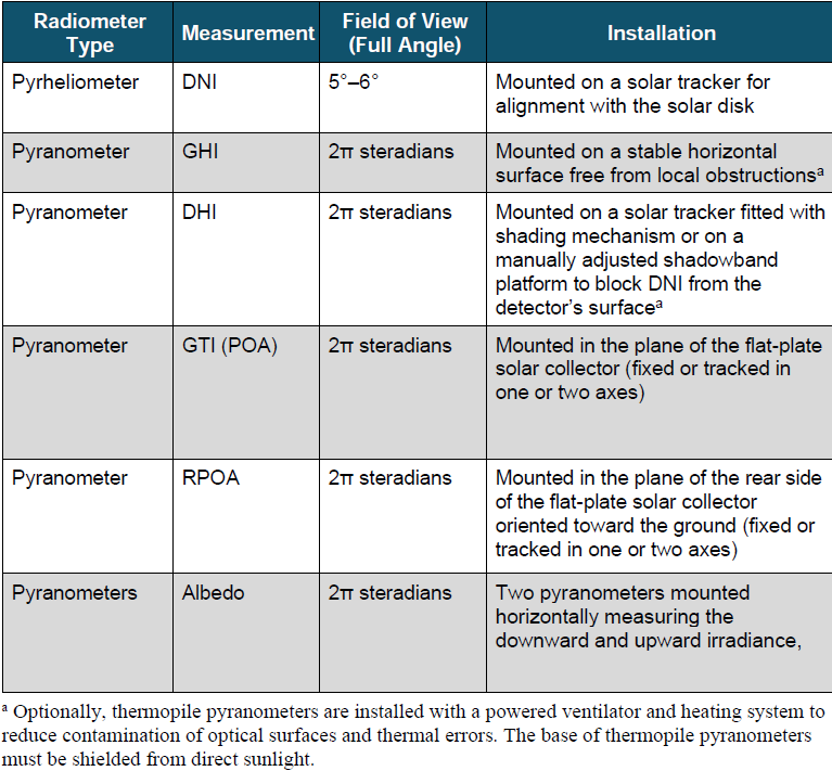
Pyrheliometers and pyranometers are two types of radiometers used to measure solar irradiance. Their ability to receive solar radiation from two distinct portions of the sky distinguishes their designs. As described earlier, pyrheliometers are used to measure DNI, and pyranometers are used to measure GHI, DHI, GTI (aka POA), or the in-plane rear-side irradiance (RPOA). Another important measurement involving pyranometers is the albedo, which can be used to estimate RHI (reflected horizontal irradiance) in Eq. (1-2b) as well as RPOA. Table 2-1 summarizes some key attributes of these two radiometers.

Table 2-1. Overview of Solar Radiometer Types and Their Applications

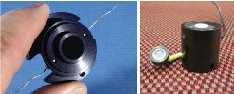
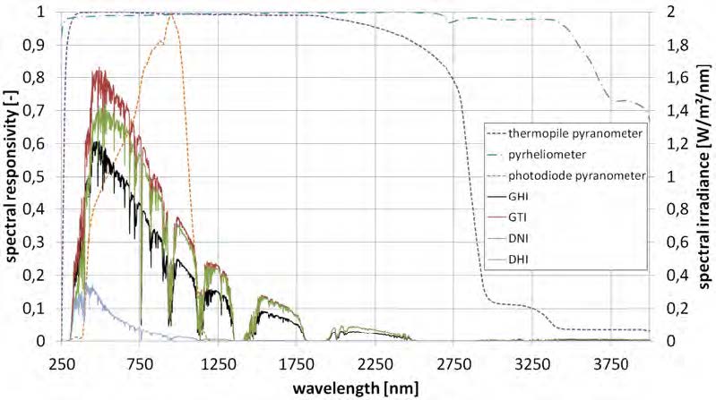
Pyrheliometers and pyranometers commonly use either a thermoelectric or photoelectric passive sensor to convert solar irradiance (W/m2) into a proportional electrical signal (microvolts [µV] DC). Thermoelectric sensors have an optically black coating that allows for a broad and uniform spectral response to all solar radiation wavelengths from approximately 300–3000 nm (Figure 2-1, left). The most common thermoelectric sensor used in radiometers is the thermopile. There are all-black thermopile sensors used in pyrheliometers and pyranometers as well as black-and-white thermopile pyranometers. In all-black thermopile sensors, the surface exposed to solar radiation is completely covered by the absorbing black coating. The absorbed radiation creates a temperature difference between the black side of the thermopile (i.e., “hot junction”) and the other side (i.e., “reference” or “cold junction”). The temperature difference causes a voltage signal. In black-and-white thermopiles, the surface exposed to radiation is partly black and partly white. In this case, the temperature difference between the black and the white surfaces creates the voltage signal. Despite having a relatively small thermal mass, their 95% response times are not negligible, and they are typically 1–30 seconds6—that is, the output signal lags the changes in solar flux. Some instruments include a signal post-processing that tries to compensate for this time lag. Recently, new smaller thermopile sensors with response times as low as 0.2 second have been made commercially available as well. A detailed analysis of radiometer response times is found in Driesse (2018).

In contrast to thermopiles, common photoelectric sensors generally respond to only the visible and near-infrared spectral regions from approximately 350–1,100 nm (Figure 2-1, right; Figure 2-2). Pyranometers with photoelectric sensors are sometimes called silicon (Si) pyranometers or photodiode pyranometers. These sensors have very fast time-response characteristics—on the order of microseconds.

For both thermopile and photelectric detectors used in commercially available instruments, the electrical signal generated by exposure to solar irradiance levels of approximately 1000 W/m2 is on the order of 10 mV DC (assuming no amplification of the output signal and an appropriate shunt resistor for photodiode sensors). This rather low-level signal requires proper electrical grounding and shielding considerations during installation (see Section 2.3.4). Most manufacturers now also offer pyrheliometers and pyranometers with built-in amplifiers and/or digital outputs. Such digital instruments can be of advantage for several reasons. Corrections for systematic errors depending on, e.g., the sensor temperature or the incident angle of the sun can be corrected directly in the instrument, which reduces the effort needed for data treatment and avoids user errors. Their implementation in a data acquisition system can be easier, and errors resulting from the transmission of low-voltage signals might be avoided. On the other hand, such digital sensors are sensitive to transients, surges, and ground potential rise, so the isolation and surge protection of power and communications lines is of high importance (Section 2.3.4).

2.2.1.1 Pyrheliometers

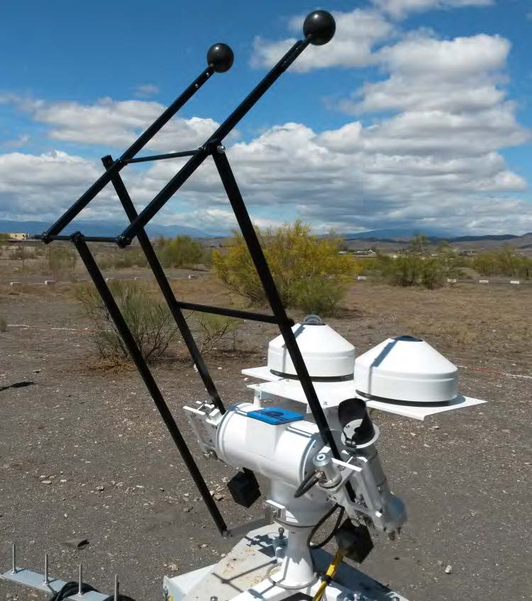
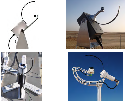
Pyrheliometers are typically mounted on automatic solar trackers to maintain the instrument’s alignment with the solar disk and to fully illuminate the detector from sunrise to sunset (Figure 2-3 and Figure 2-4). Alignment of the pyrheliometer with the solar disk is determined by a simple diopter—a sighting device in which a small spot of light (the solar image) falls on a mark in the center of a target located near the rear of the instrument, serving as a proxy for alignment of the solar beam to the detector. The tracking error is acceptable as long as the solar image is at least tangent to the diopter target. Modern sun trackers use software to compute and precisely track the sun position. These calculations require that the sun tracker is assembled and positioned correctly (horizontally levelled, correct azimuth orientation), and tracking errors occur if the tracker is not installed and positioned correctly. Tracking errors caused by imperfect levelling vary with the sun position. Sun sensors can help to reduce the remaining tracking errors during periods with no direct irradiance; hence, they are used in high-quality stations. The sun sensor is tracked to the sun and uses a four-quadrant sensor placed behind a pinhole or a lens to detect the tracking error. The tracking error is then sent to the tracker software so that it can be corrected. By convention—and to allow for small variations in tracker alignment—view-limiting apertures inside a pyrheliometer allow for the detection of radiation in a narrow annulus of sky around the sun (WMO 2018), called the circumsolar region. This circumsolar radiation component is the result of forward scattering of radiation near the solar disk, itself caused by cloud particles, atmospheric aerosols, and other constituents that can scatter solar radiation. All modern pyrheliometers should have a 5° field of view (FOV), following the World Meteorological Organization (WMO) (2018) recommendations. The FOV of older instruments could be larger, however, such as 5.7°–10° full angle. Depending on the FOV—or, to be more precise, the sensor’s penumbra function and tracker alignment, pyrheliometer measurements include varying amounts of circumsolar irradiance contributions to DNI. Although this is usually a very small contribution to the measurement, under atmospheric conditions of high scattering, it can be measurable, or even significant.

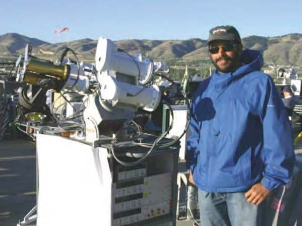
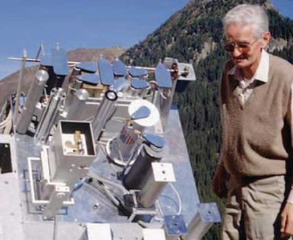
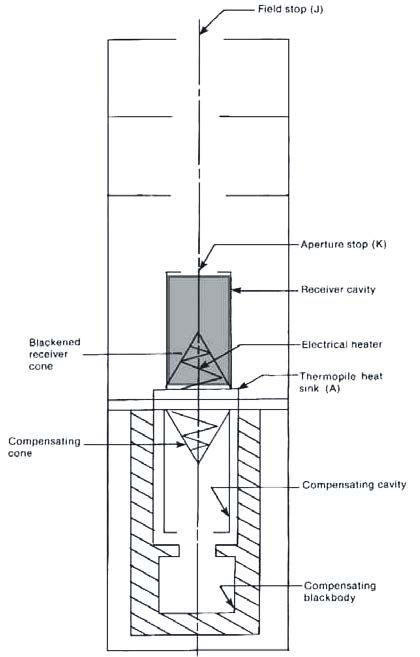
The most accurate measurements of DNI under stable conditions are accomplished using an electrically self-calibrating absolute cavity radiometer (ACR; see Figure 2-5). This advanced type of radiometer is the basis for the World Radiometric Reference (WRR), the internationally recognized detector-based measurement standard for DNI (Fröhlich 1991). The WMO World Standard Group of ACRs is shown in Figure 2-6. By design, ACRs have no windows and are therefore generally limited to fully attended operation during dry conditions to protect the integrity of the receiver cavity (Figure 2-7). Removable windows and temperature-controlled all-weather designs are available for automated continuous operation of these radiometers; however, the installation of a protective window nullifies the “absolute” nature of the DNI measurement. The window introduces additional measurement uncertainties associated with the optical transmittance properties of the window (made from either quartz or calcium fluoride) and the changes to the internal heat exchange resulting from the sealed system. Moreover, ACRs need some periods of self-calibration during which no exploitable measurement is possible. This creates discontinuities in the high-accuracy DNI time series that could be measured with windowed ACRs, unless a regular pyrheliometer is also present to provide the necessary redundancy (Gueymard and Ruiz-Arias 2015). Combined with their very high cost of ownership and operation, this explains why ACRs are rarely used to measure DNI in the field.

A unique 10-month comparison of outdoor measurements from 33 pyrheliometers, including ACRs, under a wide range of weather conditions in Golden, Colorado, indicated that the estimated measurement uncertainties at a 95% confidence interval ranged from ±0.5% for windowed ACRs to +1.4%/–1.2% for commercially available instruments (Michalsky et al. 2011). The results also suggested that the measurement performance during the comparison was better than indicated by the manufacturers’ specifications.

2.2.1.2 Pyranometers

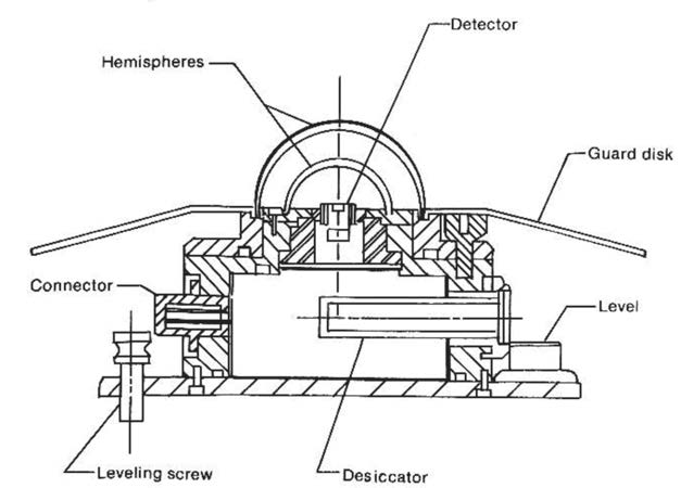
A pyranometer has a thermoelectric or photoelectric detector with a hemispherical FOV (360° or 2π steradians) (see Figure 2-4 and Figure 2-8). This type of radiometer is mounted horizontally to measure GHI. In this horizontal mount, the pyranometer has a complete view of the sky dome.

Ideally, the mounting location for this instrument is free of natural or artificial obstructions on the horizon. Alternatively, the pyranometer can be mounted at a tilt to measure GTI, e.g., in the case of latitude-tilt or 1-axis tracking systems, or vertically for building applications. In an upside-down position, it measures the ground-reflected irradiance. The local albedo is simply obtained by dividing the latter by GHI.

The pyranometer detector is mounted under a protective dome (made of precision quartz or other high-transmittance optical material) and/or a diffuser. Both designs protect the detector from the weather and provide optical properties consistent with receiving hemispheric solar radiation. Pyranometers can be fitted with ventilators that constantly blow air—sometimes heated—from under the instrument and over the dome (Figure 2-9). The ventilation reduces the potential for contaminating the pyranometer optics caused by dust, dew, frost, snow, ice, insects, or other materials. Ventilation and heating also affect the thermal offset characteristics of pyranometers with single all-black detectors (Vignola, Long, and Reda 2009). The ventilation devices can require a significant amount of electrical power (5–20 W), particularly when heated, adding to the required capacity for on-site power generation in remote areas. Both DC and AC ventilators exist, but current research indicates that DC ventilators are preferable (Michalsky, Kutchenreiter, and Long 2019).

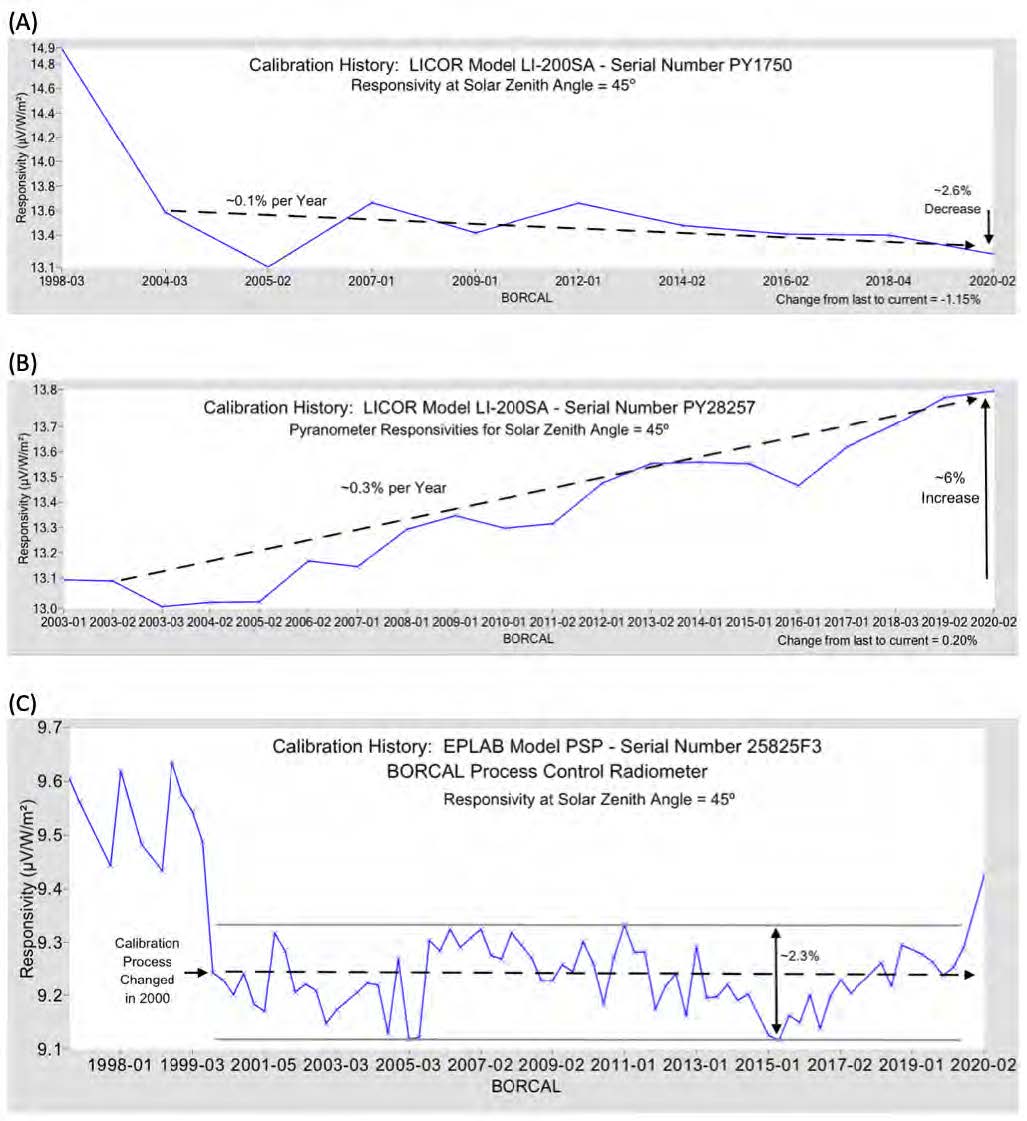
Photodiode pyranometers provide the signal in the form of a photodiode’s short-circuit current. The fast response of such photodiode pyranometers makes them interesting for some applications, e.g., the measurement of cloud enhancement or ramping events. Photodiode pyranometers employ a diffuser above the detector (Figure 2-10) to achieve an approximate hemispherical response and to omit the glass dome to reduce cost. The application of a diffuser as an external surface compared to transparent glass domes makes such pyranometers measurably more dust tolerant than pyranometers with optical glass domes (Maxwell et al. 1999). The long-term stability of photodiode pyranometers can vary differently from thermopile-based pyranometers, as shown in Figure 2-11 and as further analyzed in Geuder et al. (2014). These instrument-specific behaviors dictate the need for regular calibrations as recommended by the manufacturers.

Pyranometers can also be used to measure the diffuse irradiance. The required device for this measurement is known as a diffusometer. It consists of a pyranometer and a shading structure that blocks the direct radiation on its way to the sensor. Shading balls, shading disks, shading rings, or shadowbands are used for that purpose. Shading balls and shading disks must track the sun, and they cover only a small part of the sky corresponding to the angular region defined for measuring DNI (normally 5°). Shading rings and shadowbands cover the complete solar path during a day as seen from the pyranometer. They are built a little bit wider to cover the sun’s path on several consecutive days so that readjustments of the shading ring position are not required every day. The shading rings and shadowbands block a significant part of sky diffuse radiation; therefore, correction functions are necessary to determine DHI from the shading device. This explains why the accuracy of such a DHI determination is less than that of a DHI measurement with a shading disk or a shading ball. Shadowbands are further described in Section 2.2.5 in connection with the RSIs.

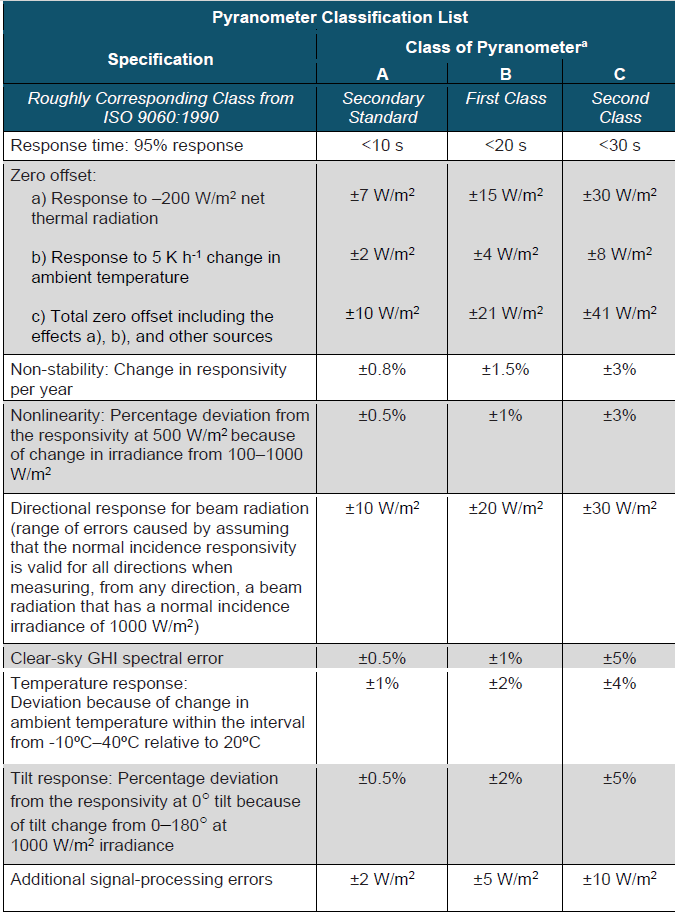
2.2.2 Pyrheliometer and Pyranometer Classifications

Both the International Organization for Standardization (ISO) and WMO have established instrument classifications and specifications for the measurement of solar irradiance. Radiometer classification can help to find the correct instrument and to interpret the data. Several instrument properties are used as the basis for these pyrheliometer and pyranometer classifications. The latest ISO specifications for these radiometers are found in ISO 9060 (ISO 2018) and are summarized in Table 2-2 and Table 2-3 based on Apogee (2019). The standard provides not only acceptance intervals but also corresponding guard bands, which is advantageous because the measurements used to obtain the sensor specifications have nonnegligible uncertainties.

The acceptance intervals provided by ISO 9060 give a general idea of the differences in data quality afforded by instrument classes; therefore, the radiometer classes can be understood as accuracy classes. The current standard also notes, however, that the acceptance intervals shown in the tables cannot be used for uncertainty calculations for measurements obtained at conditions that are different from those defined for the classification. For example, the temperature response limits are defined for the interval from -10°C to 40°C relative to the signal at 20°C. A measurement at 10°C will be connected to a different temperature response error than a measurement at 0°C or even -20°C. For the other parameters, the same principle applies. In particular, the spectral clear-sky irradiance error used for the classification can deviate from the spectral irradiance error for other conditions, e.g., cloudy conditions or other air masses. For pyranometers, it must also be considered that the spectral error for diffuse or tilted radiation is different from the spectral error for global horizontal radiation. A more detailed discussion of the clear-sky spectral error can be found in Wilbert et al. (2020).

The most important changes in the current ISO 9060 compared to the previous version, from 1990 (ISO 1990a), are as follows:

• Simple names are used for the classes (AA, A, B, C), and a new class is introduced mainly for ACRs.
• The clear-sky spectral error is used to classify the spectral properties of the radiometers, allowing photodiode-based radiometers to be also included in the ISO classification. Previously, the spectral selectivity was used, which excluded photodiode radiometers. The spectral selectivity is defined by ISO as the deviation of the spectral responsivity from the average spectral responsivity between 0.35–1.5 µm.
• Additional radiometer classes are defined relatively to their response time and their spectral responsivity. If the 95% response time is less than 0.5 second, the radiometer can be called a “fast response radiometer.” Similarly, “spectrally flat radiometers” are defined using the spectral selectivity. If a radiometer has a spectral selectivity less than 3%, it can be called a spectrally flat radiometer.
• For Class A pyranometers, individual testing of temperature response and directional response is required.
• The final signal of a sensor can be used for classification after the application of specific correction functions (e.g., for temperature response) if these corrections are applied within the measurement system (processor within instrument or control unit). Processing errors are also used as a classification criterion.

Including photodiode radiometers was considered helpful because only fast (µs) photodiode sensors can be used for accurate monitoring of extremely rapid fluctuations of solar irradiance. Under such circumstances—typically caused by cloud enhancement events—side-by-side thermopile and photodiode radiometers can disagree by a significant margin (Gueymard 2017a, 2017b). Because the most accurate way to determine GHI involves the combination of DNI and DHI measurements (ISO 2018; Michalsky et al. 1999), the shading balls, shading disks, shading masks, and rotating shadowbands used in RSIs are also defined in the current ISO 9060.

The WMO characteristics of operational pyrheliometers and pyranometers are presented for three radiometer classifications:

1. High quality: near state of the art, suitable for use as a working standard, maintainable only at stations with special facilities and staff
2. Good quality: acceptable for network operations
3. Moderate quality: suitable for low-cost networks where moderate to low performance is acceptable.

Table 2-2. ISO 9060:2018 Specifications Summary for Pyrheliometers Used to Measure DNI

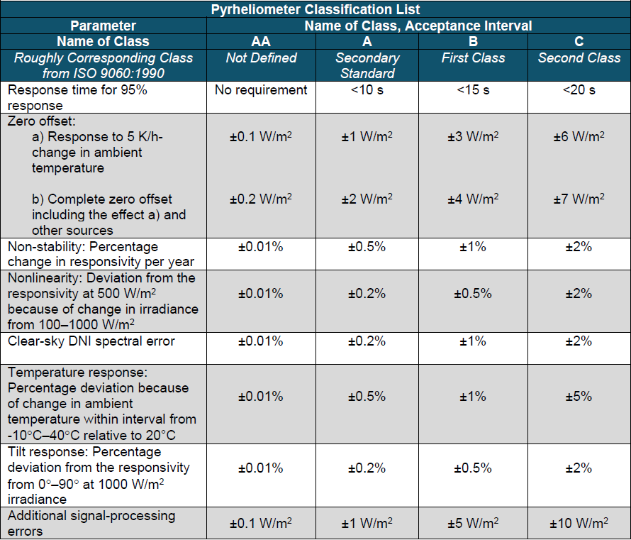
Table 2-3. ISO 9060:2018(E) Specifications Summary for Pyranometers

The WMO characteristics are similar to the classifications presented in the previous version of ISO 9060. The difference between the WMO and the outdated ISO 9060 classification is in the definition of spectral selectivity. The wavelength range used in the WMO definition is from 300–3000 nm; whereas it was from 350–1500 nm in the 1990 version of ISO 9060. The WMO limits for the selectivity for the different classes were the same or even stricter as in the case of the highest pyranometer class. This led to the unfortunate situation that, apparently, no weatherproof pyrheliometer fulfills the requirements of the WMO classes even though the spectral errors of Class A field pyrheliometers are small. (Clear-sky spectral errors are approximately 0.1%
[Wilbert et al. 2020]). Typical pyranometers of the highest class in ISO 9060 are also excluded from the WMO classification (Wilbert et al. 2020). This is true for both the 1990 and the 2018 versions of the standard; therefore, it is currently not recommended to use the WMO classification but instead to work with the most recent version of ISO 9060.

Even within each instrument class, there can be some measurement uncertainty variations. The user should research various instrument models to gain familiarity with the design and measurement performance characteristics in view of a particular application (Myers and Wilcox 2009; Wilcox and Myers 2008; Gueymard and Myers 2009; Habte et al. 2014). Further, the accuracy of an irradiance measurement depends on the instrument itself as well as on its alignment, maintenance, data logger calibration, appropriate wiring, and other conditions and effects that degrade performance.

2.2.3 Pyrheliometer and Pyranometer Calibrations

As stated, the signal of field radiometers is a voltage or a current that is ideally proportional to the solar irradiance reaching the detector. A calibration factor is required to convert the current or voltage to a solar irradiance. The calibration factor, Ccal, is the inverse of the responsivity, Rs. For example, the responsivity of a thermopile pyrheliometer is given in µV per W/m2. The irradiance, E, can be obtained from the voltage signal, Vpyr, or from the instrument’s responsivity as:

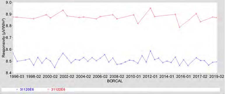
These calibration factors can vary over time, which requires periodic recalibrations, as demonstrated by the time-series plot of calibration responsivities of two pyrheliometers shown in Figure 2-12. The instability can be caused by changes in the instrument, the meteorological conditions at the time of calibration, the stability of the calibration reference radiometer(s), the performance of the data acquisition system, and other factors included in the estimated uncertainty of each calibration result.

The calibration of pyrheliometers and pyranometers is described in detail in international standards ASTM G167-05, ASTM E816-05, ASTM E824-05, ASTM G183-05, ISO 9059, ISO 9846, and ISO 9847. The calibration methods described in ISO 9846 (ISO 1993) for pyranometers and in ISO 9059 (ISO 1990b) for pyrheliometers are based on simultaneous solar irradiance measurements with test and reference instruments. ISO 9847 (ISO 1992) describes pyranometer calibrations using a reference pyranometer. These standards will be revised in the next years by the corresponding ISO working groups.

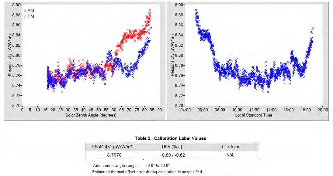
Pyrheliometers are calibrated following ISO 9059 by comparing the voltage signal of the tracked test pyrheliometer to the reference DNI from one or a group of reference pyrheliometers. For each simultaneous measurement pair, a preliminary responsivity can be calculated as the ratio of the test instrument’s voltage to the reference DNI (Figure 2-13, right). After rejecting outliers and data collected during unstable conditions, an average responsivity can be determined. Because some pyrheliometers show a noticeable correlation with the solar zenith angle (SZA), specific angular responsivities can also be derived (Figure 2-13, left and bottom). For this calibration method, it is important that clouds do not mask the sun or the circumsolar region. The calibration can be affected if significant levels of circumsolar radiation prevail during the calibration. This risk increases with the instrument’s FOV; hence, Linke turbidities should be less than 6 according to the standard method. The Linke turbidity coefficient, TL, is a measure of atmospheric attenuation under cloudless conditions. It represents the number of clean and dry atmospheres that would result in the same attenuation as the real cloudless atmosphere. One method to derive the Linke turbidity from DNI is presented in Ineichen and Perez (2002).

As mentioned, the WRR must be used as the traceable reference for the calibration of all terrestrial broadband radiometers, as stipulated by the internationally accepted Système International (SI). This internationally recognized measurement reference is a detector-based standard maintained by a group of electrically self-calibrating absolute cavity pyrheliometers at the World Radiation Center (WRC) by the Physical Meteorological Observatory in Davos, Switzerland. The present accepted inherent uncertainty in the WRR is ±0.3% (Finsterle 2011). All radiometer calibrations must be traceable to the WRR, but that does not mean that all radiometers are calibrated directly against the WRR. The calibration chain from the WRR to a field instrument can have several steps. For example, reference ACRs are used as national and institutional standards, and these instruments are calibrated by comparison to the WRR during international pyrheliometer comparisons conducted by the WRC once every 5 years. Pyranometers calibrated against traceable WRR reference pyrheliometers make these pyranometer calibrations traceable to the WRR.

Pyranometers can be calibrated outdoors with three different methods. One option, as described in ISO 9846, is to compare the DNI output from a reference pyrheliometer to that derived from the test pyranometer using the shade-unshade method. The successive voltages, Vunshade and Vshade, are proportional to GHI (unshaded) and DHI (shaded), respectively. Using the reference DNI and the relationship between GHI, DHI, and DNI, as described by Eq. (1-2a), the responsivity, Rs, of the pyranometer under test for one measurement sequence can be derived:

This method is described in more detail by Reda, Stoffel, and Myers (2003).

For this calibration method, virtually constant atmospheric conditions during the pair of shaded and unshaded measurements are required. Cloud cover must be very low, and the angular distance between clouds and the sun must be high. In addition to cloud cover, aerosol and water vapor variations could affect the calibration. This explains why only data collected for a low TL (less than 6) should be used for the calibration.

Another option offered by ISO 9846 consists of comparing the voltage signal of the test pyranometer obtained in the GHI measurement position to the GHI calculated from the DNI and DHI measurements of a reference pyrheliometer and a shaded reference pyranometer. The Rs of a pyranometer under calibration for one simultaneous set of three measurements can be computed from their unshaded signal (Vunshaded):

Computing the Rs this way is called the “component-summation calibration technique.” Again, TL should be less than 6, and a high angular distance of clouds from the sun should exist during the whole calibration period.

The third option to calibrate pyranometers outdoors is described in ISO 9847. It compares a test pyranometer to a reference pyranometer while both sensors are in the same measurement position (either GHI or GTI). The Rsi is then obtained as the ratio of the test signal to the reference irradiance. For outdoor pyranometer calibrations using a reference pyranometer (ISO 1992), the sky conditions are less precisely defined than for the other methods described. The calibration interval is adjusted depending on the sky conditions.

The indoor calibration methods from ISO 9847 use irradiance measurements under an artificial light source. For the first option, measurements are taken simultaneously after ensuring that the test and the reference pyranometer receive the same irradiance from an integrating sphere. This is done by switching pyranometer positions during the calibration procedure. The other option is to take consecutive measurements by mounting the test and the reference instrument one after the other in the same position under a direct beam. The indoor calibrations are carried out in a controlled environment that is independent from external meteorological conditions. If measurements with the reference and test pyranometer are made after each other, however, instabilities of the artificial light source increase the calibration uncertainty compared to outdoor calibrations. If simultaneous measurements are used, an additional uncertainty contribution comes from the fact that the test and the reference pyranometer might not receive exactly the same irradiance from the artificial light source, though some of this error can be mitigated by switching the positions of the instruments during the calibration procedure. Further, the incident angle of the radiation is usually not well defined for indoor calibrations. Because of the pyranometer’s directional errors (see Table 2-3), this is another source of calibration uncertainty; therefore, in general, thorough outdoor calibrations with accurate reference instruments have lower uncertainties than indoor calibrations.

The shade/unshade and component summation techniques, when conducted throughout a range of SZA, show that pyranometer responsivities are correlated with it. The variation of Rs as a function of SZA is like a fingerprint or signature of each individual pyranometer (Figure 2-14).

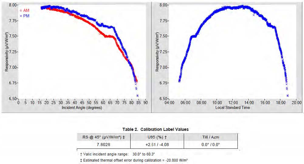
This means that the angular responsivities of different specimens of the same model can differ. Variations of pyranometer Rs can be symmetrical with respect to solar noon, or they can be highly skewed, depending on the mechanical alignment of the pyranometer, detector surface structure, and detector absorber material properties. To improve the accuracy in the GHI measurement, using an SZA and azimuth angle-dependent calibration factor for each individual measurement are recommended. This method, however, is applicable only to conditions with high direct radiation contribution to the GHI because the variation of responsivity with SZA is mostly caused by direct radiation and the associated cosine error. For situations when thick clouds mask the sun or for DHI measurements, the angular distribution of the incoming irradiance cannot be approximated well by one incidence angle. For DHI measurements, it is recommended to use the Rs for a 45° incidence angle.

For accurate photodiode pyranometer calibration, further considerations beyond these standards are necessary because of the uneven spectral response. A specific calibration method is discussed in Section 2.2.5 for RSI instruments.

2.2.4 Correction Functions for Systematic Errors of Radiometers

Some pyrheliometer and pyranometer measurement errors are systematic and can be reduced by applying correction functions. An example is the correction of the directional errors, as mentioned. Some manufacturers provide one calibration constant for a pyranometer and additional correction factors for different intervals of SZA. This treatment of the incidence angle dependence has the same effect as using an incidence-angle-dependent responsivity.

Moreover, an additional temperature correction can be applied if the internal temperature of pyranometers or pyrheliometers is measured using a temperature-dependent resistor close to the sensor. Correction coefficients are often supplied by the manufacturer.

Measurements from only black (as opposed to black-and-white) thermoelectric pyranometers can be corrected for the expected thermal offset using additional measurements from pyrgeometers (Figure 2-4, right). Pyrgeometers allow for the determination of the downward longwave irradiance between approximately 4.5–40 µm, based on their sensor (thermopile) signal and body temperature. The thermopile is positioned below an opaque window that is transparent only to the specified infrared radiation wavelength range while excluding all visible, near- infrared, and far-infrared radiation. Most pyrgeometers must be positioned below a shading ball or disk to limit window heating by DNI. Ventilation units are also used for pyrgeometers, as in the case of pyranometers. If no pyrgeometer is available, a less accurate correction for the thermal offset can be made based on estimations of the thermal offset from the typically negative measurements collected during the night (Dutton et al. 2000; Gueymard and Myers 2009).
Correction functions for photodiode pyranometers are presented in Section 2.2.5.2.

2.2.5 Systems for Determining Solar Irradiance Components

A measurement system that independently measures the basic solar components—GHI, DNI, and DHI—will produce data with the lowest uncertainty if the instruments are properly installed and maintained. Alternatives exist to reduce the overall cost of such a system while offering potentially acceptable data accuracies, depending on the application. These alternatives are designed to eliminate the expense and complexity of an automatic solar tracker with pyrheliometer and shaded pyranometer.

2.2.5.1 Rotating Shadowband Irradiometers
RSIs use a fast detector that is periodically shaded by a motorized shadowband, which rapidly sweeps back and forth across the detector’s FOV (Figure 3-15). The principle of operation of these RSIs is to measure GHI when unshaded and DHI when shaded. The DNI is calculated using the fundamental closure equation relating these three components, Eq. (1-2a):

RSIs are often called rotating shadowband radiometers (RSRs) or rotating shadowband pyranometers (RSPs), depending on the instrument manufacturer. RSI refers to all such instruments measuring irradiance by use of a rotating shadowband. There are two types of RSIs: RSIs with continuous rotation and RSIs with discontinuous rotation.

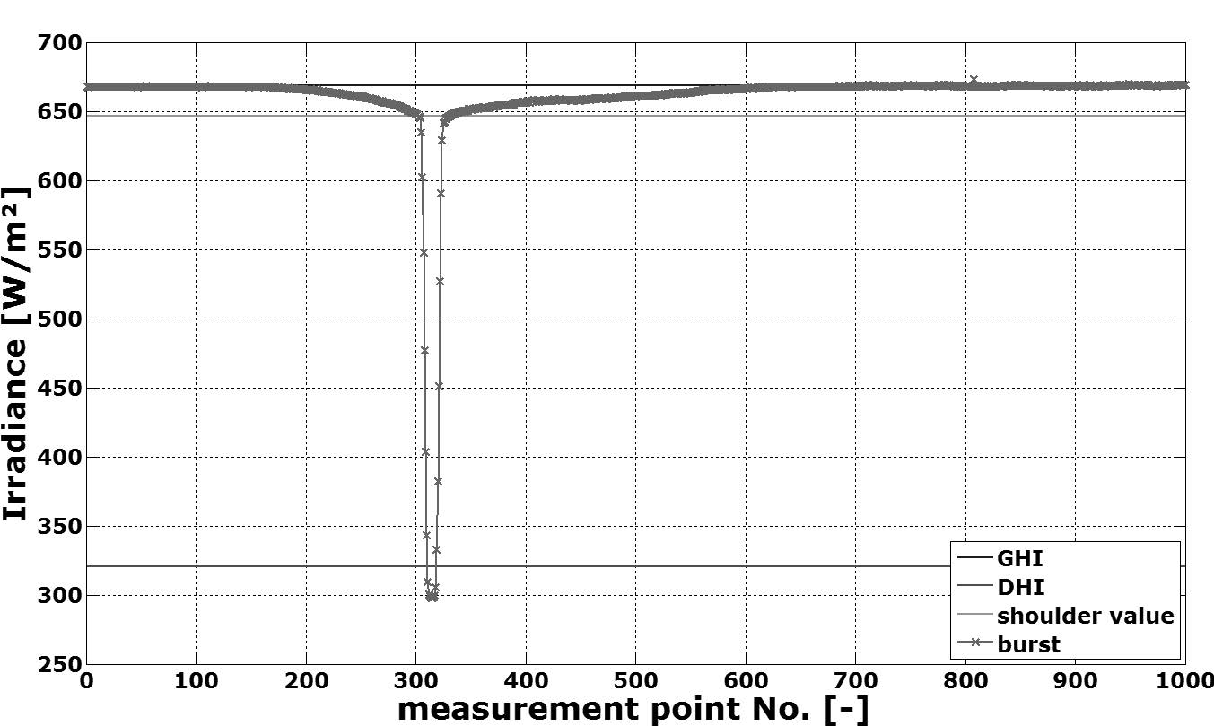
The operational principle of RSIs with continuous rotation is shown in Figure 2-16. At the beginning of each rotation cycle, the shadowband is below the pyranometer in its rest position. The rotation is performed with constant angular velocity and takes approximately 1 second. During the rotation, the irradiance is measured with a high and constant sampling rate
(approximately 1 kHz). This measurement is called a burst or sweep. At the beginning of the rotation, the pyranometer measures GHI. The moment the center of the shadow falls on the center of the sensor, it approximately detects DHI; however, the shadowband covers some portion of the sky, so the minimum of the burst is less than DHI. Thus, so-called shoulder values are determined by curve analysis algorithms. Such algorithms are usually implemented in the data logger program and use the maximum of the absolute value of the burst’s slope to find the position of the “shoulder values.” The difference between GHI and the average of the two shoulder values is added to the minimum of the curve to obtain the actual DHI. Subsequently, DNI is calculated by the data logger using GHI, DHI, and the SZA calculated by the known time and coordinates of the location, as stated. All the RSIs shown in Figure 2-15 (except for the SDR-1 model) work with a continuous rotation.

RSIs with discontinuous rotation do not measure the complete burst but only four points of it. First, the GHI is measured while the shadowband is in the rest position. Then the shadowband rotates from the rest position toward the position just before it begins shading the diffuser, stops, and a measurement is taken (e.g., during 1 second for the SDR-1 shown in Figure 2-15). Then it continues the rotation toward the position at which the shadow lies centered on the diffuser, and another measurement is taken. The last point is measured in a position at which the shadow has just passed the diffuser. The measurement with the completely shaded diffuser is used equivalently to the minimum of the burst, as shown in Figure 2-16. The two measurements for which the shadow is close to the diffuser are used equivalently to the shoulder values to correct for the portion of the sky blocked by the shadowband.

These two types of RSIs have advantages and disadvantages. An RSI with continuous rotation needs a detector with a fast response time (much less than 1 second—e.g., approximately 10 µs). Because thermopile sensors cannot be used, photodiodes are used instead—typically using Si. An example is the Si-based radiometer model LI-200SA shown in Figure 2-11. Because of the nonhomogeneous spectral response of such Si sensors (see Figure 2-2), the measurement accuracy of highest class thermopile pyranometers cannot be reached. Correction functions for this and other systematic errors must be applied to reach the accuracy required in resource assessments, albeit still not on par with the accuracy of thermopile instruments. These correction functions are discussed in Section 2.2.5.2.

RSIs with discontinuous rotation need sufficiently long measurement times for each of the four points to allow the use of a thermopile detector (e.g., the Yankee TSR-1 thermopile shadowband radiometer, now discontinued); thus, the spectral error of a photodiode can be avoided—at least partly. So far, RSIs with discontinuous rotation typically rely on a diffuser, which has its own uneven spectral transmittance over the shortwave spectrum; hence, the spectral error of such RSIs cannot be neglected. Further, the discontinuous rotation is connected to other disadvantages compared to the continuous rotation. Although RSIs with continuous rotation are not affected by small azimuth alignment errors (within approximately ±5°), the azimuth alignment of RSIs with discontinuous rotation is crucial for their accuracy. Moreover, the accuracy of the sensor’s coordinates and sweep time is more important for the discontinuous rotation. If the shadowband stops in the wrong position, the DHI measurement is incorrect. Further, the duration of the measurement with a discontinuous rotation increases the measurement uncertainty. This is especially relevant if the RSI uses a thermopile sensor and if sky conditions are not stable (e.g., cloud passages). If GHI and the sky radiance distribution change during the four-point measurement, the data used to determine DHI will be inconsistent. In contrast, this complication is less relevant for continuously rotating RSIs because their rotation takes approximately only 1 second.

DHI is typically determined one or four times per minute, but GHI measurements can be sampled at a higher frequency whenever the shadowband does not rotate—for example, every second. The temporal variation of GHI also contains some information about any concomitant change in DNI. Different algorithms are used to determine the averages of DHI and DNI between two DHI measurements using the more frequent GHI measurements. Temporal variation detected by the higher frequency GHI measurement can be used to trigger an additional sweep of the shadowband to update the DHI measurement under rapidly changing sky conditions.

The initial lower accuracy of RSIs compared to ISO 9060 first-class pyrheliometers and secondary standard pyranometers is often compensated by some unique advantages of RSIs. Their simplicity/robustness, low soiling susceptibility (Pape et al. 2009; Geuder and Quaschning 2006; Maxwell et al. 1999), low power demand, and comparatively lower cost (instrumentation and O&M) provide significant advantages compared to thermopile sensors and solar trackers, at least when operated under the measurement conditions of remote weather stations, where power and daily maintenance requirements are more difficult and costly to fulfill.

With neither correction of the systematic deviations nor a matched calibration method, under the best field circumstances RSIs yield an uncertainty of only 5%–10%. This accuracy is notably improved, to approximately 2%–3%, with proper calibration and the application of advanced correction functions (Wilbert et al. 2016), which are described in the following sections. Most instrument providers also offer post-processing software or services that include these correction functions. Users should ask the manufacturer whether such post-processing is part of the instrument package and is readily available.

Because of the stated disadvantages of RSIs with discontinuous rotation and the higher relevance of RSIs with continuous rotation for solar energy applications, the focus here is on RSIs with Si photodiodes and continuous rotation. More information about RSIs with discontinuous rotation can be found in Harrison, Michalsky, and Berndt (1994).

2.2.5.2 Correction Functions for Rotating Shadowband Irradiometers
The main systematic errors of RSIs with photodiode sensors are caused by the spectral response of the detector, its cosine response, and its temperature dependence.
Several research groups have developed correction functions that reduce systematic errors in RSI readings. In all cases, the photodiode of the RSI is a LICOR LI-200SA. Whereas temperature correction is similar in all versions (King and Myers 1997; Geuder, Pulvermüller, and Vorbrügg 2008), the methods for the spectral and cosine corrections vary.

Alados-Arboledas, Batlles, and Olmo (1995) used tabular factors for different sky clearness and skylight brightness parameters as well as a functional correction depending on SZA. King and Myers (1997) proposed functional corrections in dependence on air mass and SZA, primarily targeting GHI. This approach was further developed by Augustyn et al. (2002) and Vignola
(2006), including diffuse and subsequently direct beam irradiance. The combination of the GHI correction of Augustyn et al. (2002) and of the diffuse correction from Vignola (2006) provides a complete set of corrections for LI-200SA-based RSIs. Independently, a method for DNI, GHI, and DHI correction was developed by the German Aerospace Agency, Deutsches Zentrum für Luft- und Raumfahrt (DLR), using functional corrections that include a particular spectral parameter obtained from GHI, DHI, and DNI (Geuder, Pulvermüller, and Vorbrügg 2008). Additional corrections in dependence on air mass and SZA were used. Another set of correction functions was later presented in Geuder et al. (2011). Additional new correction methods are on their way (Vignola et al. 2017; 2019; Forstinger et al 2020). An overview of RSI correction functions can be found in Jessen et al. (2017).

2.2.5.3 Calibration Methods for Rotating Shadowband Irradiometers
In addition to the corrections mentioned, special calibration techniques are required for RSIs. As of this writing, RSIs with continuous rotation are equipped with LI-200SA or LI-200R pyranometers. They come with precalibration values from the manufacturer (LI-COR) for GHI based on outdoor comparisons with an Eppley precision spectral pyranometer (PSP) with an accuracy stated as better than 5% (LI-COR Biosciences 2005). Considering that the PSP has only limited performance (Gueymard and Myers 2009), an additional calibration (e.g., on-site or with respect to DHI, DNI, or GHI independently) of the RSIs can noticeably improve their accuracy (Wilbert et al. 2016).

Because of the rather narrow and inhomogeneous spectral response of the photodiodes and the combined measurement of DHI and GHI, only some aspects of the existing ISO standards for pyrheliometer and pyranometer calibrations can be transferred to RSI calibration. Calibrating RSI instruments involves independently field-calibrating them for DNI, DHI, and GHI. Each of these three steps is challenging because each irradiance component has a distinct spectral composition that can change during the day or from one location to another. Because of the spectral response of the Si detectors and/or the diffusers, it is problematic to calibrate an RSI based on only a few short series of measurements. This is possible for thermopile sensors because of their homogenous spectral response covering at least 300–3000 nm (which amounts to >99% of the ASTM G173 DNI spectrum). A similar calibration method of RSIs would need the spectra during the calibration and the additional—but incorrect—assumption that all RSIs from a single manufacturer have exactly the same nominal spectral and cosine response. Then the RSI measurements obtained later in a resource assessment station could be described by nominal correction functions and estimated or measured spectra. A similar approach using a calibration period of several weeks was tested in Forstinger et al. (2020), but it is still not applied for solar projects. Because of the possible variations between the spectral response of different pyranometers of the same model, using separate calibration constants for at least two of the three components (GHI, DHI, and DNI) is recommended; however, some RSI calibration methods include only GHI calibration. The current best practice is to consider a long enough calibration period to include the wide variety of meteorological conditions that are expected at the site where the RSI is planned to be used. Such conditions should be assessed and characterized wisely during the calibration process. The calibration accuracy generally improves when the atmospheric conditions during the calibration closely represent those at the site where the RSI is intended to be operated later, though in reality such conditions will be highly variable. In addition to cloud cover, the effects of aerosols, water vapor, and site altitude on the solar spectrum must be considered (Myers 2011; Wilbert et al. 2016). Calibrations with artificial radiation sources that lack the spectral power distributions of natural solar radiation components usually also lack the variety of natural irradiation conditions; therefore, field calibrations under natural irradiation conditions should yield more accurate calibrations and are thus preferable.
Outdoor RSI calibrations are performed at only a few laboratories, such as the National Renewable Energy Laboratory (NREL), in Golden, Colorado; and DLR at CIEMAT’s (Centro de Investigaciones Energéticas, Medioambientales y Tecnológicas) Plataforma Solar de Almería in Spain. Additionally, on-site calibrations are performed by a few specialized companies. At the Plataforma Solar de Almería, for instance, RSIs are operated parallel to ISO-9060 Class-A pyrheliometers and pyranometers under real-sky conditions (Figure 2-17). The duration of RSI calibrations is from several hours to more than 1 year. These longer calibration periods provide a database for the analysis of systematic signal deviations and measurement accuracy. An analysis of the dependence of the calibration constants on the duration of the calibration period, as well as more details on two possible calibration methods, are presented in Jessen et al. (2016) and Geuder, Affolter, and Kraas (2012). Data quality is analyzed and compared to the reference irradiances. RSI calibrations are performed according to the different methods described. All published calibration techniques are based on the comparison of corrected RSI signals (using the existing correction functions described) to reference irradiance measurements obtained with thermopile sensors.

Depending on the calibration method, one, two, or even three calibration constants are defined. The motivation for determining one calibration constant is that only one pyranometer is used and the calibration based on GHI is less time-consuming than performing separate calibrations for GHI, DHI, and DNI. Because of the Si detector’s spectral response, the spectral sensitivities for DHI, GHI, and DNI are not the same; hence, the application of two or three calibration constants is physically reasonable, even though only one sensor is used.

Examples of drift in the GHI calibration constants obtained from Geuder et al. (2008) were later investigated for nine sensors in Geuder et al. (2016) and Jessen et al. (2016). For recalibration periods from 2–3.75 years, changes in this GHI calibration constant were less than 1% in most cases. Recalibration is recommended at least every 2 years. An overview of current RSI calibration methods is presented in Jessen et al. (2016), and more details can be found in Geuder et al. (2008, 2016) and Kern (2010).

The calibration techniques for RSIs can be partially used for other solid-state radiometers. Further details on RSIs and RSI-specific measurement best practices can be found in Wilbert et al. (2015).

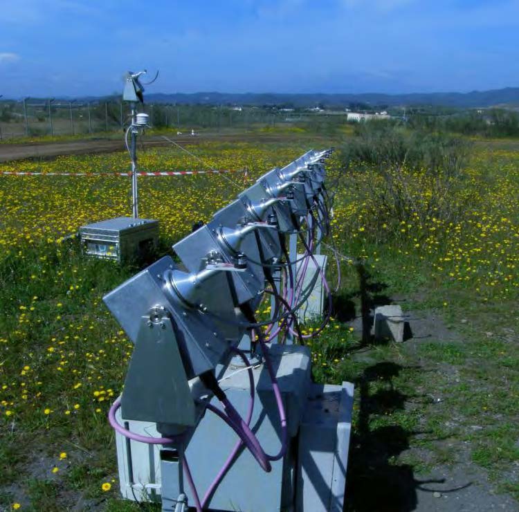
2.2.5.4 Other Instruments Used to Derive Diffuse Horizontal Irradiance and Direct Normal Irradiance
In addition to the radiometers described above, other instruments can be used to derive DHI or DNI from irradiance measurements. For example, the scanning pyrheliometer/pyranometer
(Bergholter and Dehne 1994, 245ff) or the sunshine duration sensor Soni e3 (Lindner 1984) can be used to derive DNI; however, these two sensors reach only lower accuracies than tracked pyrheliometers, thermopile pyranometers with shading balls, or even RSIs, as documented in Geuder et al. (2006). Note that researchers have developed methods for estimating daily integrated values of DNI from the vast archive of measurements from Campbell-Stokes sunshine recorders (Stanhill 1998; Painter 1981).

Another option for DNI measurements without tracking is the EKO MS-90 instrument (Figure 2-18), which is based on an earlier sunshine recorder sensor (MS-093). The revised design uses a rotating mirror within a fixed glass tube tilted to latitude (–58° to +58°). The mirror reflects the direct beam onto a broadband pyroelectric detector that senses DNI four times per minute. Preliminary tests were conducted against a reference pyrheliometer (EKO MS-57) during the North American Pyrheliometer Comparison held at NREL in September 2016. The tests showed rather small deviations for a simple nontracking instrument when DNI exceeds 600 W/m2.

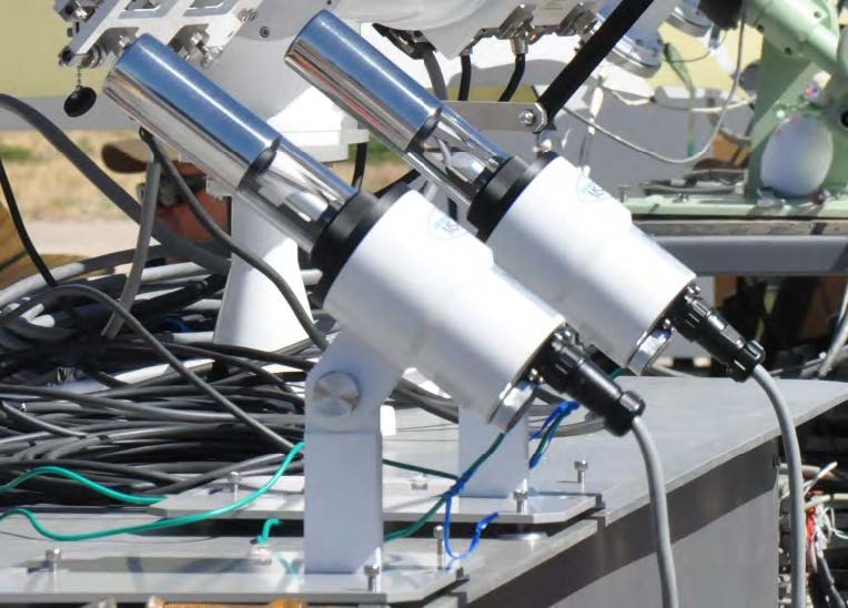
Recently, all-sky imagers have also been used to measure solar irradiance (Kurtz and Kleissl 2017). The accuracy of such measurements alone is still too low for their application in resource assessment. Another option for estimating DNI from measurements of both DHI and GHI by a single instrument is the SPN1 (Figure 2-19).

The SPN1 consists of an array of seven fast-response thermopile radiation detectors that are distributed in a hexagonal pattern under a glass dome. The detectors are positioned under diffuser disks and a special hemispherical shadow mask. The shape of the mask is selected such that for any position of the sun in the sky there is always one or more detectors that are fully shaded from the sun and exposed to approximately half the diffuse radiance (for completely overcast skies). Also, one or more detectors are exposed to the full solar beam for all positions. The minimum and the maximum readings of the seven detectors are used to derive GHI and DHI.

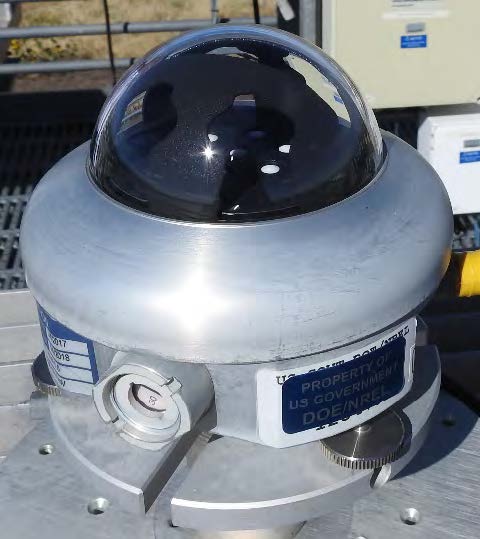
With this principle of operation, GHI, DHI, and DNI can be derived without any moving parts and without needing alignment other than horizontal leveling. Further, the SPN1’s low power demand (the temperature-controlled dome prevents dew and frost) increases its suitability for operation in remote sites compared to DNI or DHI measurements involving solar trackers. Test results indicate that the accuracy of the SPN1’s GHI is comparable with RSIs, but its DNI and DHI readings have higher errors than the DNI measured with RSIs (Vuilleumier et al. 2012). Further, SPN1 performance results obtained at six different locations worldwide can be found in Badosa et al. (2014). An additional comparison with traditional radiometers is presented by Habte et al. (2016).

2.2.6 Photovoltaic Reference Cells for Outdoor Use

The photodiode detectors in the photoelectric pyranometers that are discussed are essentially tiny PV cells, usually only several square millimeters, and their operating principle is identical to the larger cells used in PV modules and PV power plants. The larger cells can also be used as radiometer elements, and when they are mounted in a suitable enclosure for measurement purposes, they are referred to as PV reference cells. Commercial products in this category are quite diverse, as shown in Figure 2-20. Their active cell area ranges from approximately 4–225 cm2 (from left to right).

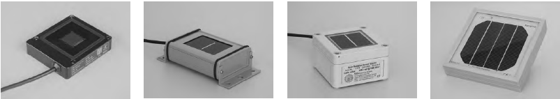
Although they can be physically diverse, PV reference cells share four main characteristics:

1. The output signal is proportional to the short-circuit current of the detector PV cell, and it is usually the voltage measured across an internal shunt resistor. The cell does not produce electrical power in this configuration, but the measured short-circuit current represents the amount of radiation that could be converted to electric power.
2. The detector PV cells are protected by a flat, transparent window, which leads to reflections at the air-window interface and consequently lower irradiance readings for beam radiation coming at higher angles of incidence. This would be considered a very poor directional response by the definition of the pyranometer classes, but it allows the reference cell readings to more closely track the power output of a PV plant—especially when the window material matches the glass used in the plant’s PV modules. Figure 3-21 shows the variations in the angular response from the four commercial reference cells.
3. Like photodiode pyranometers, the spectral response of PV reference cells is narrow and nonuniform (Figure 2-22). This leads to a high spectral error according to the terms of the pyranometer classification, but, again, it allows the reference cells to track the PV plant output more closely. This works best when the technology of the reference cell—and hence its spectral response—matches that of the modules in the PV plant. In some reference cells, a filter glass is used to absorb some of the near-infrared light before it reaches the silicon detector (PV cell), thereby creating an overall spectral response that more closely matches another cell type, such as amorphous silicon or cadmium telluride.

   

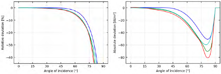
4. In practice, the output signal has a pronounced positive temperature dependency. This dependency is primarily a by-product of the spectral response and therefore varies by technology (it is approximately 400–500 ppm/K for crystalline silicon cells); however, it is not the same as the effect of temperature on PV module power output, which decreases with temperature. Reference cell products nearly always include a temperature sensor, and they could offer temperature-corrected or uncorrected irradiance signals as output.

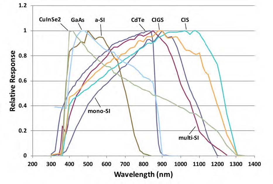
Note that this course focuses on PV reference cells designed for long-term continuous outdoor measurements. Products outside this category could differ substantially—for example, certain reference cells for indoor use only do not have a protective window. It is also possible to use a regular full-sized PV module as a radiometer by measuring its short-circuit current; however, this is also out of scope.

It is clear from these descriptions that reference cells are fundamentally different from the other types of radiometers discussed in this course. These differences are not intrinsically good or bad, but rather they influence which type of radiometer is best suited for a given measurement objective. PV reference cells are not intended to measure broadband hemispherical irradiance; in fact, some product designs would collect water when mounted horizontally, thus yielding large errors. If a low-cost substitute for a thermopile pyranometer is needed, a photodiode pyranometer is a usually better choice.

2.2.6.1 Standardization of Photovoltaic Reference Cells
Because of their measurement characteristics, reference cells are not consistent with ISO or WMO pyranometer classifications (ISO 2018; WMO 2018). Although many standards apply to PV reference cells directly or indirectly, there is no standard akin to ISO 9060 that would describe precisely and completely how reference cells should behave. In other words, there exists a definition of an ideal pyranometer but not of an ideal reference cell. Nevertheless, IEC 60904-2:2015 – Part 2 (IEC 2015) provides many useful requirements (e.g., linearity better than 0.5% and acceptance angle >160°) and recommendations for reference devices ranging from single cells to whole modules. One of the most important aspects of this standard is the extensive documentation requirement, which states that calibration reports must include spectral responsivity, temperature coefficient, and many other details about the device itself as well as the calibration method and equipment used. Currently, most manufacturers of PV reference cells for outdoor use do not claim to apply this standard.
There is also a de facto World Photovoltaic Scale (WPVS) reference cell standard. This was first established in 1997 by a group of laboratories seeking to establish a reference scale similar to the WRR (Osterwald et al. 1999). WPVS cells conform to IEC 60904-2 and fulfill several very specific additional design criteria (e.g., physical dimensions and connections) that improve long-term stability and repeatability of measurements. Their high cost is more easily justified in a laboratory setting than for fieldwork; nevertheless, outdoor versions of WPVS cells are available.

2.2.6.2 Calibration of Photovoltaic Reference Cells
The responsivity of PV reference cells varies with wavelength, intensity and direction of the incident light, and the temperature of the cell. The calibration value is the response of the device (usually a value in millivolts) under a precisely defined spectral irradiance: the AM1.5 global spectrum (IEC 60904-3, IEC (2019a)) with irradiance 1000 W/m2; and with a device temperature of 25°C. Combined, these conditions are referred to as the standard test conditions (STC), which apply equally to PV module ratings. Reference cell response is normally linear with irradiance; therefore, the value of the response under STC is equal to the responsivity of the device in mV per 1000 W/m2 or µV/(W/m2).

IEC 60904-4:2019 – Part 4 (IEC 2019b) describes four different methods to perform the calibration of primary reference devices with traceability to SI units, so the relationship of reference cells to broadband radiometers is well defined. All these methods consider the narrow spectral response of PV devices by calculating a spectral mismatch factor, which compensates for the fact that the light used during calibration does not normally correspond precisely to the AM1.5 global reference spectrum.

IEC 60904-2:2019 – Part 2 describes how secondary or field reference cells can be subsequently calibrated by comparison to a primary reference device using either natural or simulated sunlight. When the spectral response of the primary reference cell is the same as that of the cell being calibrated, there is no spectral mismatch to be considered.

Primary reference cells are usually calibrated at precisely 25°C so that no temperature correction is required, and when identical devices are used for secondary or field calibrations, the effect of temperature cancels out. When there are differences in devices or device temperatures, however, a correction must be done as part of the calibration. Measurement procedures to determine the temperature coefficient are covered by IEC 60891 (IEC 2009); essentially, they consist of measuring the response over a range of temperatures and determining the slope of a linear fit.

In all calibration situations, the direction of the incident light is predominantly normal to the plane of the cell, implying little or no diffuse irradiance. This minimizes the influence of the directional dependence, but in recent work this aspect has been analyzed more comprehensively, and the use of an angular mismatch factor has been proposed to further improve calibration consistency (Plag et al. 2018).

In the context of calibrations, any adjustments for temperature, spectrum, or direction tend to be small compared to the effects of temperature, spectrum, and direction on field measurements.

2.2.6.3 Deployment Considerations
Because of the four distinct characteristics of PV reference cells, the natural place to deploy them would be in the context of PV projects. The benefit of the application of reference cells in solar resource assessment depends on the technology and the project phase. The benefits of reference cells for a resource assessment before the power plant construction are different from those for PV plant monitoring. The similarity of a PV reference cell to a specific PV technology can be of advantage if this PV technology is used, but other PV technologies will require a different reference cell, and solar thermal systems will require broadband measurements.

For planning large power plants, satellite data sets are adapted to the site using ground measurements to achieve the required high accuracy. Traditionally, the available irradiance data was broadband and collected using pyranometers, pyrheliometers, RSIs, or other devices, as described; hence, only broadband irradiance is provided by most satellite data sets, and broadband ground measurements are required for their validation and site adaptation. Only a few satellite-derived data sets include spectral data (Müller et al. 2012; Xie and Sengupta 2018), and such data are not available for the full globe.

Another application of ground measurements collected before the plant construction is PV plant modeling. PV power plant models include effects such as reflectance losses and spectral mismatches to derive the power output from the broadband irradiance. Modeling these effects is related to additional errors, and the reference cells could offer an attractive alternative: If irradiance is measured under a flat glass cover, the reflectance losses do not need to be modeled; and if the irradiance measurement is already weighted by the spectral response of the reference cell, then no spectral correction model is required. In other words, if a PV reference cell is used, then the expected PV system output can be calculated with substantially fewer modeled steps, avoiding the uncertainty those would contribute; therefore, including a tilted reference cell in a ground measurement station is of interest before the plant construction. One drawback for the use of reference cells before actual plant construction is that the exact technology that will be used in the power plant might not be known at the beginning of the measurement campaign. Deviations among the temperature, incidence angle, and spectral effects of different PV products could be bigger than the uncertainty of the PV simulation models for these effects; hence, different reference cells should be used if the PV technology has not been selected before a measurement campaign. Another important limiting factor for the application of reference cells for PV system modeling is the available software used for PV yield simulations. Most do not accommodate selectively bypassing certain model calculation steps, which would be required for adequate use of PV reference cell irradiance measurements. If such a limited software is used, it imposes to some extent the use of a broadband pyranometer.

For PV monitoring, the advantages of PV reference cells are already much clearer, even without significant further research and development. The described accuracy enhancement is of great interest for PV monitoring and capacity testing. The limitation due to the PV system modeling tools also affects this application if a model using pyranometer-based GTI measurement is contracted for the monitoring; however, PV models used for PV monitoring or capacity testing more frequently allow the application of reference cell measurements as input than models used before the PV plant is built. Moreover, measurements with both pyranometers and reference cells are of interest. In the case of bifacial PV modules, spectrally matched reference cells are also an option to measure the required rear-side irradiance. To measure the rear-side irradiance, the reference cells are mounted on the module racking with an adequate support structure so that they are exposed as similarly as possible as the modules. End row effects are avoided and depending on the size of the PV plant and the variation of the ground and shading properties, several sensors must be used.

To conclude, PV reference cells can be a helpful source of solar resource data, especially for PV monitoring, but currently they cannot replace broadband measurements in the context of general solar resource assessments. It is possible, however, that new, improved resource assessment methods will evolve that are specialized for PV applications and rely primarily on PV reference cells.
General considerations for the instrument selection and the selection of the radiation components that should be measured are presented in Section 2.3.5.

2.2.6.4 Recent and Ongoing Research
The key to the effective use of PV reference cells is to understand their special characteristics and to apply that knowledge when collecting, interpreting, and using the data they produce. One active area of research is to quantify these characteristics for product categories, product models, and individual instruments (see Figure 2-23) (Driesse et al. 2015; Vignola et al. 2018). Directly related to this are studies attempting to apply this knowledge of characteristics to instrument calibration, uncertainty analysis, and modeling (Driesse and Stein 2017).
Although complete knowledge of PV reference cell characteristics is desirable, it is not always practical to acquire and use it, even if it is available. Parallel and complementary efforts are underway to promote increased homogeneity and further standardization (Habte et al. 2018).

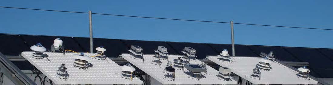
2.3 Measurement Station Design Considerations

To collect useful solar resource data, the successful design and implementation of a solar resource measurement station or a network of stations requires careful consideration of the elements summarized in this section. The measurement stations also include additional meteorological instrumentation, such as anemometers, wind vanes, thermometers, and hygrometers. The general recommendations—such as station security and data logging—described in this section also apply to these instruments.

2.3.1 Location

The primary purpose of setting up a solar resource measurement station before the construction of a solar power plant is to collect data that will ultimately allow an analyst to accurately characterize the solar irradiance and relevant meteorological parameters at that specific location. Ideally, the instruments would be within the targeted analysis area. In some cases, however, separation distances might be tolerated depending on the complexities of local climate and terrain variations. Less variability in terrain and climate generally translates to less variability in the solar resource over larger spatial scales. These effects should be well understood before determining the final location of a measurement station. The proximity to the target area must be weighed against operational factors, such as the availability of power, communications, and access for maintenance, as discussed in this chapter. Considerations should also include the possible effects of local sources of pollution or dust—for example, traffic on a nearby dirt road that could impact the measurements.

Solar radiation measurements are also required for medium or large power plants. Further, measurements can be helpful for other solar energy purposes, such as testing power plant components or for PV power forecasting for many small PV systems. In power plants and for component or system tests, the position of the station must be such that the measurements reflect the conditions of the power system as well as possible. In large power plants, this means that several distributed stations can be required. For PV systems, IEC 61724-1:2017 defines the number of required radiometers within the PV power plant depending on the system’s peak power.

When measurement stations are constructed in metropolitan areas, industrial areas, or near electrical substations or solar power plants, consideration should be given to possible sources of radio frequency signals and electromagnetic interference that could impart unwanted noise in sensors or cables. For example, the same high building that could provide an attractive unobstructed site for solar measurements could also be the ideal location for radio or television broadcast towers or some other apparatus. Such sites should be investigated for interference with the irradiance sensors and monitoring station. See Section 2.3.4 for additional information regarding proper shielding and grounding.

Instrument placement is also an important consideration. If nearby objects—such as trees or buildings—shade the instruments for some period during the day, the resulting measurement will not truly represent the available solar resource in a nearby unshaded part of the site. Distant objects—especially mountains—could be legitimate obstructions because the shadows they cast are likely to produce an influence beyond the area local to the instruments. Conversely, nearby objects can potentially reflect solar radiation onto the instruments, resulting in measurements that do not represent the conditions for the power plant. Such cases could include a nearby wall, window, or other highly reflective object. The best practice is to locate instruments far from any objects that are in view of the instrument detector. The recommendations from WMO (2018) for radiation apply, if not mentioned otherwise.

The easiest way to determine the quality of solar access is to scan the horizon for a full 360° of azimuth and note the elevation of any objects protruding into the sky above the local horizon. Look for buildings, trees, antennae, power poles, and even power lines. Most locations will have some obstructions, but whether they will be significant in the context of the necessary measurements must be determined. Camera-based devices can be used to assess any obstructions including far shading from mountains, trees, etc., and the assessment can be easily documented and quantified, such as seasonal shade effects. Generally, pyranometers are insensitive to sky blockage within approximately 5° elevation above the horizon. Pyrheliometers, however, are more sensitive because objects can completely block DNI, depending on the daily path of the sun throughout the year. The duration and amount of daily blockage are related to the object’s width and height above the horizon. On an annual basis, the number of blockage days depends on where along the horizon the object lies. To be a concern, the object must be in the area of the sun near sunrise or sunset, the time and azimuth of which vary throughout the year. For most of the horizon, objects blocking the sky will not be a factor because the sun rises in a limited angular range in the east and sets likewise in the west during sunset (e.g., at 40° N latitude, sunrise occurs approximately 60° from true north at the summer solstice and 120° from true north at the winter solstice). The farther north in latitude the site is located, however, the greater the angular range of these sunrise and sunset areas of interest. A solar horizon map, or even a sketch of obstructions by elevation and azimuth, will help determine the areas where horizon objects will affect the measurement (see Figure 1-5). Such maps can be created with digital cameras and software. Several commercial products using curved mirrors and also apps for smartphones exist.
Considerations for locating a station should also include environmental factors, such as wildlife habitat, migratory paths, drainage, and antiquities or archeological areas.

2.3.2 Station Security and Accessibility

Measurement stations can cost tens of thousands or even hundreds of thousands of dollars. Although this equipment is typically not the target of thieves seeking property for resale, it is still subject to theft and should be protected. Vandalism might be even more likely than theft. The less visible and accessible the station is to the public, the less likely it will be the target of theft or vandalism. For example, instruments mounted on a rooftop are less likely to attract unwanted attention than those unprotected beside a highway. Lack of visibility is the best defense against vandalism.

Security fences should be used if people or animals are likely to intrude. Within a fenced solar power plant, no additional fences are required. Fencing should be at least 1.8-m tall, preferably with barbed wire and fitted with locking gates in high-profile areas where intrusion attempts are likely. Less elaborate fences might suffice in areas that are generally secure and where only the curious need to be discouraged from meddling with the equipment. In remote venues with few human hazards, cattle fence paneling (approximately 1.2-m tall) might be advisable if large animals roam the area. The fencing should be sturdy enough to withstand the weight of a large animal that might rub against the compound or otherwise be pushed or fall against the fence. It might not be possible to keep smaller animals out of the station compound, and precautions should be taken to ensure that the equipment, cabling, and supports can withstand encounters with these animals. Rodents, birds, and other wildlife could move through the wires or jump over or burrow under fences. Signal cabling between modules or sensors at or near ground level is prone to gnawing by rodents and should be run through a protective conduit or buried. Any buried cable should be either specified for use underground or run through conduit approved for underground use. Underground utilities and other objects should be investigated before postholes are dug or anchors are sunk.

If fences are used, they must be considered a potential obstacle that could shade the instruments or reflect radiation to the instruments. The radiometers should be positioned at least above the line between the horizon and the fence (including barbed wire), if only by a few millimeters, to prevent any shading of the sensor. This assumes that the pyranometer is mounted in a horizontal position and that the pyrheliometer is installed on a solar tracker. Tilted pyranometers should have an unobstructed view of the ground and sky in front of them. For albedo measurements, fences cause measurement errors if the area under the downward-facing pyranometer is shaded. This must be considered for the station design. The recommendations from WMO (2018) concerning obstacles should be followed. Deviations between WMO (2018) and the actual station design are acceptable if these deviations affect not only the measurement station but also the solar energy system that is analyzed using the measurements. If nearby towers are unavoidable, the station should be positioned between the tower and the equator (e.g., to the south of the tower in the northern hemisphere) to minimize shading. The radiometers should be positioned as far as possible from the tower—at least several meters—so the tower blocks as little of the sky as possible. Nevertheless, radiometer signal cables should be shorter than 50 m to avoid losses caused by line resistance. The tower should also be painted a neutral gray to minimize strong reflections that could contaminate the solar measurement. These guidelines assume that the tower is part of the measurement station proper and that the site operator has control of the placement or modification of the tower. Without that control, the radiometers should be placed as far as possible from the tower.

Access to the equipment must also be part of a station’s construction plan. Because routine maintenance is a primary factor affecting data quality, provisions must be made for reasonable and easy access to the instruments. Factors here could include ease of access to cross-locked property, well-maintained all-weather roads, and roof access that could be controlled by other departments. Safety must also be a consideration. Locations that present hazardous conditions—such as rooftops without railings or that require access using unanchored ladders—must be avoided.

2.3.3 Power Requirements

Ongoing measurements require a reliable source of electrical power to minimize system downtime from power outages. In some areas, power from the utility grid is reliable, and downtime is measured in minutes per year. In other areas, multiple daily power interruptions are routine. Depending on the tolerance of the required analysis to missing data, precautions should be taken to ensure that gaps in the data stream from power outages do not seriously affect the results. The most common and cost-effective bridge for power outages is an uninterruptible power supply (UPS). The UPS can also filter out unwanted or harmful line voltage fluctuations that can occur for a variety of reasons. It has internal storage batteries that are used as a source of power in case of an AC power interruption. When the AC power is interrupted, internal circuitry makes an almost seamless switch from grid-connected AC power to AC provided through an inverter connected to the battery bank. When power is restored, the UPS recharges the internal battery from the AC line power. Power loss is detected quickly, as is switching to the battery, and it is measured in milliseconds or partial line cycles. Some equipment could be particularly susceptible to even millisecond power interruptions during switching and should be identified through trial and error to avert unexpected downtime despite use of the UPS.

The UPS is sized according to:

• Operating power: How much can it continuously supply either on or off grid-connected AC power?
• Operating capacity: How long can the UPS supply power if the grid connection is interrupted?

Users should estimate the longest occurring power outage and size the UPS for the maximum load of attached devices and the maximum period of battery capacity. Batteries should be tested regularly to ensure that the device can still operate per design specifications. This is most important in hot areas (such as deserts) because batteries could overheat and become inoperative (temporarily or permanently). Internal battery test functions sometimes report errors only when batteries are near complete failure and not when performance has degraded. A timed full-power-off test should be conducted periodically to ensure that the UPS will provide backup power for the time needed to prevent measurement system failure.

In remote locations where utility power is not available, local power generation with battery storage should be devised. Options for on-site electrical power generation include PV or small wind turbine systems (or both) and gasoline- or diesel-fueled generators. The renewable energy systems should be sized to provide enough energy for the maximum continuous load and power through several days of adverse conditions (cloudy weather and/or low wind speeds). This includes sites prone to persistent surface fog. The sizing is a function of the extremes of the solar climate and should consider the longest gap during reduced generation, the shortest recharge period available after discharge, and the generation capacity and storage necessary to provide uninterrupted power for the target location. Some oversizing is necessary to accommodate degradation of PV panels and battery storage, and consideration should be given to ambient temperature, which affects the ability of a battery to deliver energy. Sizing calculators are available to help with this effort.7

Equipment should be specified and tested for self-power-on capability in the event of a power outage. This ensures that when power is restored, the equipment will automatically resume measurements and logging without operator intervention. This is an important consideration for remote locations where considerable downtime might occur before personnel can be dispatched to restart a system.

2.3.4 Grounding and Shielding

Station equipment should be protected against lightning strikes and shielded from radio frequency interference that could damage equipment or reduce the validity of the measurements. Several references are available that describe techniques for grounding and shielding low-voltage signal cables (see, e.g., Morrison 1998). Those designing solar resource measurement systems are urged to consult these references and seek expert technical advice. If digital sensors with onboard analog-to-digital converters are used, their sensitivity to transients, surges, and ground potential rise must be considered; therefore, the power and communications lines should be isolated and surge protected with physical isolation, surge protection devices, or other equivalent technology.

In general, the following steps should be taken when designing and constructing a measurement station:

1. Use a single-point ground (e.g., a copper rod driven several feet into the ground) for all signal ground connections to prevent ground loops that can introduce noise or biases in the measurements.
2. Use twisted pair, shielded cables for low-voltage measurements connected as double- ended measurements at the data logger. Double-ended measurements require separate logger channels for + and – signal input conductors. These inputs are compared to each other; therefore, the possibilities for electrical noise introduced in the signal cable are significantly reduced.
3. Physically isolate low-voltage sensor cables from nearby sources of electrical noise, such as power cables. Do not run signal cables in the same bundle or conduit as AC power cables. If a power cable must cross a signal cable, always position the two at right angles to each other. This case is not recommended, but this limited contact will minimize the possibility of induced voltages in the signal cable. Also, the data logger settings should be selected to avoid signal noise (the integration time of the voltage measurement adjusted to AC frequency).
4. Connect metal structures such as masts and tripods to the ground to provide an easy path to the ground in the event of a lightning strike. This will help protect sensitive instruments. Electronic equipment often has a special ground lug and associated internal protection to help protect against stray voltages from lighting strikes. These should be connected with a heavy gauge wire to ground (12 American wire gauge or larger). Metal oxide varistors, avalanche diodes, or gas tubes can be used to protect signal cables from electrical surges such as lightning. These devices must be replaced periodically to maintain effectiveness. The replacement frequency is a function of the accumulated energy dissipated by the unit. The U.S. National Electric Code recommends a ground resistance of less than 5 Ohms for “sensitive” electronic equipment. If that cannot be met with one rod, multiple rods should be used and bonded together. Ground resistance should be measured with a ground resistance tester using the three-pin or four-pin method.

2.3.5 Measurement and Instrument Selection

From among the descriptions, the station designers should choose the instrumentation and the radiation components that will best support the data and uncertainty goals of the project. As discussed, station designers must consider not only the accuracy under optimum maintenance conditions but also the expected accuracy for the likely maintenance conditions. Depending on the project phase, different instruments could be used.

Before constructing large power plants, radiation measurements are used mainly to enhance the accuracy of satellite-derived long-term data sets with different site adaptation methods. For concentrating technologies, only the DNI resource is ultimately of interest, and hence in principle only a pyrheliometer would be needed. This minimalist setup is not recommended, however, because the best data quality control methods rely on the independent measurement of the three radiation components (see Section 2.4.2). For fixed non-concentrating techniques, such as most PV plants, measuring GHI would be the minimal option because long-term GHI data can be site-adapted with the GHI measurement and then converted to POA with decomposition and transposition models. Measuring only GTI on a tilt corresponding to the anticipated POA is not advisable because long-term data sets typically do not provide GTI and because site adaptation methods have only been developed for DNI, GHI, and DHI. Although such minimalistic measurement setups with only one instrument might seem sufficient at first, it is advantageous and hence common to measure further radiation components or to include redundant sensors for the same component. There are several reasons for this. Measuring multiple radiation components in one station increases the accuracy of yield predictions, improves the detection of measurement errors, and gives more flexibility regarding the selection of the power plant technology.

The accuracy of PV yield calculations can be increased by measuring not only GHI but also DNI or DHI. Transposition models used to derive GTI from GHI and DNI are much more accurate than decomposition and transposition models that derive GTI from GHI alone. With only the DNI or DHI measurement available at a site, the DNI satellite data can be enhanced with the ground measurements. For more detailed PV system simulations, ground measurements are helpful as direct input. With GHI and DNI data, the PV simulations are more accurate because one can consider that mainly the direct component is affected by incidence angle and shading.

Additional GTI measurements are advantageous for resource assessment because they can be used to select the best transposition (or decomposition and transposition) model for the site. One must consider that the best transposition (and decomposition) model for open field measurements, however, might not be the best option once the plant is built because the modules affect the incoming radiance distribution. GTI measurements are more accurate than modeled GTI and can be used as direct input for detailed PV modeling. One complication for GTI measurements is selecting the right orientation and tilt of the POA pyranometer before starting the measurement campaign. The optimal orientation depends on the latitude, the meteorological conditions at the site, the shading effects, and the electricity market, among others. Tracked POA measurements might also be of interest, and deploying reference cells should also be considered (Section 2.2.6.3). Reference cells can be valuable for such additional measurements.

A further advantage of radiometers is related to the quality control of the data and to the detection of errors. If global, direct, and diffuse irradiance are known, it is possible—though not advisable—to measure two of the three because the third parameter can be calculated from the other two. The most accurate installations include all three components. This provides not only redundancy in case of instrument failure but also—and more importantly—the basis for the most rigorous data quality protocols, as described in Section 2.4.2. Also, redundant measurements of the same radiation component can be of interest to avoid data gaps and increase accuracy.

Measuring the three radiation components with a solar tracker, a pyrheliometer, a pyranometer, and a shaded pyranometer induces a significant maintenance effort. Without trained personnel providing daily cleaning and prompt corrections in case of tracker or alignment errors, data gaps and increased uncertainties are common. Measurements of DNI or DHI, however, in addition to that of GHI, are recommended for both tracked and fixed utility-scale PV projects and of course also for concentrating collectors; therefore, simple, more robust instruments, such as RSIs

(section 2.2.5), at times in combination with a thermopile pyranometer, can be a better option to determine the three radiation components. In this case, only a less effective quality control, as in the case of measurements with two radiometers (e.g., GHI and DNI), is possible because of the principle of operation of these radiometers.

The third main advantage of measuring several radiation components is the increase in flexibility for the selection of the solar technology. The exact technology option or mix might not be selected at the start of the measurement campaign. Depending on the site conditions, tracked PV could be an advantage over fixed PV. If tracked PV is used, DNI measurements are more important than they are for fixed PV systems. A concentrating solar power (CSP) project could be less adequate than PV for a specific site—for example, because of higher than expected aerosol load, which reduces DNI much more than GTI. If PV is selected instead of CSP, GTI must be measured or modeled.
Additional radiometers add to the instrumentation budget, but when considering the overall costs of acquiring the property, building the infrastructure, providing long-term labor for O&M, and underwriting the resources required for processing and archiving, the added cost is nominal, and its inclusion will likely pay off with a valuable dimension of credibility for the project and the associated reduced financing costs.

To operate solar power plants, different measurements are required. For PV, the International Electrotechnical Commission (IEC) standard 61724-1 (IEC 2017) defines the parameters to be measured for PV monitoring. GTI and GHI measurements are required for the highest accuracy level defined in the standard. Depending on the peak power of the PV system, different numbers of sensors of the same type are required. The IEC standard also defines the instrument types allowed in the classes. PV monitoring Class A systems use the highest ISO 9060 class pyranometers or reference cells with low uncertainty. For PV monitoring Class B systems, less accurate pyranometers and reference cells are allowed. Class B can be of interest for small- or medium-size power plants. For bifacial PV systems, rear-side irradiance and/or albedo must also be measured, according to a revision of the standard that is currently under preparation. For CSP, no standard is available that defines the instrumentation that should be used at the power plant; however, virtually all CSP plants use ISO 9060 Class-A pyrheliometers to measure DNI. GHI and DHI are not specifically mentioned, but this is a disadvantage because of the reduced ability to quality-control the radiation measurements. At present, there is no consensus on the required number of DNI measurements per CSP plant. In some instances, only one pyrheliometer is used; whereas in other plants, four or more DNI measurements are taken.

Apart from the radiation measurements, other meteorological parameters are required for resource assessment and during the operation of a solar power plant.

2.3.6 Data Loggers

Most radiometers output a voltage, current, or resistance that is measured by the data logger, which comprises a voltmeter, ammeter, and/or ohmmeter. The measured output value is subsequently converted to the units of the measurand through a multiplier and/or an offset determined by calibration to a recognized measurement standard.

Data loggers should be chosen to have a very small measurement uncertainty, perhaps 3–10 times smaller than the estimated measurement uncertainty associated with the radiometer. This is the accuracy ratio between the data logger and the radiometer. For example, typical specifications for a good data logger measuring a 10-mV output from the radiometer accurate to 1%, or 0.1 mV (100 µV), are on the order of total uncertainty (accuracy) of better than (less than) 0.1% of reading (or full scale) for the parameter in question, which would be 0.010 mV, or 10 µV.

The logger should also have a measurement range that can cover the signal at near full scale to best capture the resolution of the data. For example, a sensor with a full-scale output of 10 mV should be connected to a logger with a range that is at least 10 mV. A logger with a 1-V range might be able to measure 10 mV but not with the desired accuracy and resolution. Most modern data loggers have several range selections, allowing the user to optimize the match for each instrument. Because of the nature of solar radiation, radiometers (e.g., pyranometers used for GHI measurements) can sometimes produce 200% or more of clear-sky readings under certain passing cloud enhancement conditions, and the logger range should be set to prevent over-ranging during these sky conditions. The absolute GHI limit that can be reached during cloud-enhancement situations is a decreasing function of the measurement time step, but this can be misleading. At a 1-minute resolution, a safe limit seems to be 1800 W/m2, but it could reach 2000 W/m2 or more at a 1-second resolution with photodiode radiometers. Because the data logger measures near-instantaneous values regardless of its averaging or recording time step, the range should be set to accommodate the higher values described. See Gueymard (2017a, 2017b) for more details.

Some radiometers use amplifiers to increase the instrument output to a higher range to better satisfy signal range matching requirements; however, such amplifiers will add system complexity and some uncertainty to the data with nonlinearity, noise, temperature dependence, or instability. High-quality amplifiers could minimize these effects and allow a reasonable trade-off between logger cost and data accuracy. Calibrations should be made of these radiometer systems by coupling the pyranometer or pyrheliometer with its uniquely associated amplifier.

The logging equipment should also have environmental specifications that are compatible with the environment where the equipment will be used. Loggers used inside an environmentally controlled building could have less stringent environmental performance specifications than one mounted outside in a desert or arctic environment. Equipment enclosures can create an internal environment several degrees above ambient air temperature because of solar heating (absorption by the enclosure materials), heat generated by electronic devices mounted inside, and the lack of sufficient ventilation to help purge heat.

The sampling rate and recording rates of the solar resource data should be determined from the desired data analysis requirements. The sampling rate refers to how often the logger measures in a time interval. The recording rate is often also called the reporting rate or the time resolution. It is the length of the time interval that is represented by one data point in the logger’s output file. Monthly averages or sums, daily, hourly, minute, or sub-1-minute data records can be of interest. Data loggers can generally be configured to produce output of instantaneous or integrated values at any reasonable time period consistent with the radiometer time-response characteristics. The design should consider the current requirements and, if convenient and practical, future needs for additional analyses. A high-temporal-resolution data-logging scheme can be down-sampled or integrated into longer time periods—but not the other way around. Data logging equipment, data transfer mechanisms, and data storage can generally handle 1-minute data resolution, and this should be considered the recording rate in the data logger. A resolution of 1 minute or better is recommended to allow for accurate data quality control. Because most applications address the solar energy available over time, integrating data of sub-minute samples within the data logger is a common method of data output regardless of the final data resolution required by the analysis. For instance, 1-second signal sampling is recommended for irradiance measurements in the Baseline Surface Radiation Network (BSRN) (McArthur 2005) so that 60 samples are averaged to the reported 1-minute data. The output of the instantaneous samples at longer intervals is much less likely to represent the available energy and should be avoided when configuring a data logger. If the size of a measured data set is a defining issue (e.g., limited data communications throughput), the user can determine the lowest temporal resolution necessary for the application and optimize the data collection accordingly.

2.3.7 Data Communications

Provisions should be made for automatically and frequently transferring data from the data logger to a data processing facility. This is the basis for adequately frequent data checks and timely corrections of outages and errors. Such frequent connections also allow for automatic data logger clock corrections when a local Global Positioning System device, which is preferred, is not available. Noticeable clock corrections of more than 1 second should never be necessary. Historically, data have been captured, transferred, and processed in various ways. Today, electronics and telecommunications allow remote data collection from nearly any location. One option uses a physical connection between logger and a computer that is used for further data analysis or that forwards the data via Internet connection. To avoid a cable connection, a cellphone network can be configured to provide virtual Internet links between a measurement station and the data center. Satellite uplinks and downlinks are also available for data transfers in areas that are not served by either wire- or cell-based phone service. Within the area of an observing station, wireless communications such as radio-frequency connectivity might be useful to minimize the need for long cables between radiometers and data loggers. Depending on the antennas, data can be transferred over distances of a few kilometers. Such distances can occur between the data logger and the control room in big solar power plants with several megawatts of electrical design power.

To prevent data loss in case of connection problems, the memory of the data logger should be selected appropriately. Memory extensions are available for many data loggers with external cards.

2.4 Station and Network Operations

The protocols and procedures dictating station operations play a fundamental role in the assurance of data quality. These procedures must be established prior to the start of data collection, and then a process must be put into place to carry forth and document adherence to the procedures. Data quality is in great part established the moment the measurement is taken. If errors occur during the measurement, little can be done to improve fundamental quality. For example, a poorly maintained station with dirty optics or misaligned instruments will produce unreliable (large uncertainties or systematic biases) data, and the magnitude of the problem is not likely to be discernable until days or weeks later. Often, one can only guess at which approximate a posteriori adjustments (if any) to make.

In this context, data quality control involves a well-defined supervisory process by which station operators are confident that when a measurement is taken with unattended instruments, the instruments are in a state that produces data of known quality. This process largely encompasses the calibration, inspection, and maintenance procedures discussed in Section 2.4.1, along with log sheets and other items that document the condition of the station. It also includes a critical inspection or assessment of the data to help detect problems not evident from physical inspection of the instruments.

When designing and implementing a data quality plan, keep in mind that eventually the data set will undergo scrutiny for quality. In the best scenario (and a scenario that is certainly attainable), a data analyst will feel comfortable with the quality of the data set and will be willing to move unhindered to the analysis at hand. The plan should eliminate as much as possible any doubts and questions about how the data were collected and whether the values they contain are suitable for the intended purpose. Implementation of the best practices contained in this course help eliminate doubts and uncertainties that might jeopardize future projects.

2.4.1 Equipment Maintenance

Proper O&M practices are essential for acquiring accurate solar resource measurements. Several elements in a chain form a quality system. Collectively, these elements produce accurate and reliable solar resource data: station location, measurement system design, equipment installation, data acquisition, and O&M practices. Proper O&M requires long-term consistency, attention to detail, complete and transparent documentation, and a thorough appreciation for the importance of preventive and corrective maintenance of sensitive equipment.

Calibrations are performed with clean instrument optics and a carefully aligned/leveled instrument. To properly apply the calibration factor, the instrument should be kept in the same condition during field measurements as during the calibration. To maintain the calibration relationship between irradiance and radiometer output, proper cleaning and other routine maintenance are necessary. All O&M should be carefully documented with log sheets or preferably with electronic databases that contain enough information to reveal problems and solutions or to assert that the instruments were in good form when inspected. The exact times of the maintenance events should be noted rather than estimated. Time-stamped pictures taken before and after maintenance with a camera can be extremely useful to evaluate the importance of soiling and misalignment, for example. A button connected to the data logger that is pressed at the beginning and at the end of an inspection is also recommended. The O&M information enables an analyst to identify potentially bad data and provides important documentation to determine and defend the overall quality of the measurements.

The maintenance process includes:

• Checking the alignment/leveling of the detector. Pyrheliometers must be accurately aligned with the solar disk for accurate DNI measurements. Pyranometer detectors must be horizontal for GHI and DHI measurements and accurately tilted (or aligned with a flat-plate collector) for GTI measurements. The radiometer orientation should be checked periodically using the features described earlier in this chapter.
• Cleaning the instrument optics. To properly measure the solar irradiance, no contaminant should block or reduce the radiation falling on the detector. The outdoor environment provides many sources of such contamination, such as dust, precipitation, dew, frost, plant matter, insects, and bird droppings. The sensors should be cleaned regularly to minimize the effect of contaminants on the measurements. In many cases, this can require daily maintenance of radiometers, especially in the case of pyrheliometers. Different standards require or recommend different cleaning frequencies between daily and weekly.
• Documenting the condition of the radiometer. For analysts to understand limitations of the data, conditions that affect the measurements must be documented. This includes substandard measurement conditions, but it is equally important to document proper operations to add credibility to the data set. Observations and notes provide a critical record of conditions that positively and negatively affect data quality.
• Documenting the environment. As a consistency check, note the sky and weather conditions at the time of maintenance. Note any ground surface changes, such as vegetation removal or the presence of snow. This information is valuable when interpreting data from the radiometer, including measurements with unusual values.
• Documenting the infrastructure. The whole measurement station should be examined for general robustness. Any defects should be noted and corrected.

Maintenance frequency depends on prevailing conditions that soil the instruments. This includes dust, rain, dew, snow, birds, and insects. It also depends on instrument type. Radiometer designs based on optical diffusers as the surface separating the inside of the instrument from the environment are less susceptible to the effects of dust contamination than instruments with clear optics, such as domed pyranometers (Myers et al. 2002). This is because fine soiling particles scatter much more than they absorb solar radiation. Absorption affects instruments with clear optics and diffusers the same way. In contrast, the scattering-induced soiling effect has less impact on instruments with diffusers because the latter can transmit most of what the particles have scattered. The scattered radiation (mostly in the forward direction) hence reaches the detector in nearly the same way that radiation would enter a clean diffuser. Conversely, the scattering often causes the incoming radiation to miss the detector in instruments with clear optics because the latter is some distance from the former. This is especially relevant for pyrheliometers (Geuder and Quaschning 2006). Soiling of windowed or domed radiometers can quickly affect their reading and increase their measurement uncertainty. This explains why thermopile radiometers must be cleaned very frequently (e.g., daily). As described earlier, using a ventilator for a pyranometer can reduce this risk of contamination; thus, it is important to consider the frequency and cost of maintenance for proper instrument specification. Although sensors with diffusers, such as RSIs, are not prone to strong soiling effects, they still require regular cleaning (e.g., twice per month). Note that a diffuser below a clear entrance

window/dome does not have an advantage compared to a thermopile below the same clear entrance window/dome.
Daily cleaning for sensors with clear optics or cleaning twice per month for sensors with diffusers as an outer surface is appropriate in most cases; however, different standards require or recommend different cleaning frequencies between daily (ISO TR9901) and weekly (IEC 61724-1). It is recommended to determine the cleaning interval for each site depending on the climate conditions of similar sites or, e.g., by analyzing the immediate effect of cleaning on the measurement signal. Depending on the noted period after which soiling significantly influences the measurement, the cleaning interval can be adjusted so that the degradation in sensitivity is limited to an acceptable level (e.g., <1% for high-quality stations). Each cleaning period and the state of the sensors should be documented, and the measurement values should be checked to evaluate the effect of cleaning on the recorded values.

Radiometers should be carefully cleaned at each inspection, even if soiling appears minimal. Cleaning is generally a very short procedure. A recommendation for the cleaning procedure is as follows. First, remove any loose particles from the entrance window with a soft brush or compressed air. Then clean the entrance window, dome, or diffuser with a dry cloth. If dirt remains after this step, wet a second cloth with distilled water (or methyl hydrate), and wipe the window/diffusor/dome clean. If ice sticks to the surface, try melting the ice with one’s hands. Avoid using a hair dryer to melt the ice because the heat can crack the cold optics. More aggressive methods might damage the entrance windows and are therefore not recommended.

Collimators without entrance windows (as used in active cavity radiometers and at least one new commercially available, low-cost pyrheliometer) greatly reduce the accumulation of dust on the sensor’s entrance optics, but they could still be affected by insects or spiders because they can enter the collimators, causing strong signal reductions. Even a single fiber of a spiderweb can significantly reduce the signal; therefore, such collimators must be inspected frequently.

At remote sites that could be too difficult to maintain during extended periods, a higher class windowed instrument might not be optimal, despite its potential for better measurements. The cost of maintenance for a remote site could dominate the estimated cost of setting up and operating a station. This aspect should be anticipated when planning a measurement campaign.

Often, less maintenance-intensive sensors with initially lower accuracy than windowed instruments can be a better choice, at least until the station becomes permanently serviceable on a sufficiently frequent basis.

Additional spot inspections should be conducted after significant weather events (e.g., dust storms, snowstorms, heavy rainfall, rainfall during periods with high aerosol loads, and storms). Radiometer optics might not necessarily soil within a 24-hour period, but the effects of soiling can be best mitigated with frequent inspection.

Maintenance at remote measurement sites away from institutional or corporate employment centers will require finding a qualified person nearby who can perform the necessary maintenance duties. The qualifications for maintenance are generally nontechnical, but they require someone with the interest and disposition to reliably complete the tasks. As a rule, compensating these people for time and vehicle mileage—rather than seeking volunteers— becomes a worthwhile investment in the long run because it sets up a firm contractual commitment to perform all necessary maintenance duties. Without that formal relationship, it can become difficult to assert the need for reliable and regular attention.

A general conclusion is that a conservative maintenance schedule will support the credibility of the measurement data set and provide the analyst with a base of justification when assigning confidence intervals for the data.

2.4.2 Data Inspection

The collection of quality data cannot occur without careful and ongoing inspection of the data stream for evidence of error or malfunction. Although the maintenance procedures discussed in the previous section rely heavily on the physical appearance of the equipment to detect malfunction, some sources of error are so insidious that they cannot be revealed by simple physical observation; thus, an operations plan must include a careful inspection of the data itself for unrealistic values that might appear only with mathematical analysis. As with the inspections during equipment maintenance, inspection of data should be done with a frequency great enough to avoid prolonged error conditions that would impose a significant bias on the eventual statistical characterization of the data set.

2.4.2.1 Data Quality Control and Assurance
A successful quality-control process requires elements of quality assessment and feedback. Figure 2-24 depicts a quality-assurance cycle that couples data acquisition with quality assessment and feedback.

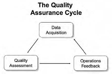
As shown in Figure 2-24, the information flows from data acquisition to quality assessment, where criteria are applied to determine data quality. The results of the quality assessment are analyzed and formed into feedback that goes back to the data acquisition module. The activities in the boxes can take several forms. For example, quality assessment could be the daily site inspection, and the analysis and feedback could be a simple procedure that adjusts the equipment malfunctions. Alternatively, the quality assessment could be a daily summary of data flags, and the analysis would then provide a determination of a specific instrument problem that is transmitted back to maintenance personnel, instructing them to correct deficiencies or to further troubleshoot problems.

The faster the cycle runs, the sooner problems will be detected. This reduces the amount of erroneous data collected during failure modes. Conversely, if the site is inspected infrequently, the chances increase that a large portion of the data set would be contaminated with substandard measurements. More than one quality-assurance cycle can—and likely will—run at any time, each with a different period and emphasis, as noted: daily inspection, weekly quality reports, and monthly summaries.

One practical aspect of this cycle is the importance of positive feedback—a regular report back to site personnel of high-quality operations. This positively reinforces a job well done and keeps site operators cognizant that data are being used and checked and that their efforts are an integral part of an ongoing process. It is often helpful to have an on-site person handle maintenance and address problems and a central facility that runs quality checks and spots potential problems with the data. Maintenance reports can advantageously include a photographic record of each radiometer, e.g., before and after cleaning or leveling.

The quality-assurance cycle is important, and thus it should be well defined and funded to maintain consistent data quality over time. After the quality of the data is determined, corresponding conclusions must be made for further use of the data. In every case, the quality-assurance data must be included in the data set as metadata. In some cases, the completeness of the data can even be improved based on the quality assurance. For example, data gaps from one sensor can be filled with the redundant data from related sensors. Gap filling is a complex topic that is not described in detail here. To calculate daily, monthly, or yearly sums, gap filling will nearly always be necessary, and it is recommended that the reader consider various publications concerning the topic for this type of correction (Hoyer-Klick et al. 2009; Espinar et al. 2011; Schwandt et al. 2014). Because data gaps can rarely be completely avoided in long time series, and because gap filling might not always work during long periods of missing data, a critical problem is then to obtain correct estimates of the long-term (e.g., monthly or annual) averages, which are of utmost importance in solar resource assessments. Practical methods have been developed to overcome this problem with the minimum possible loss of accuracy, as described by Roesch et al. (2011a, 2011b). But in the context of this section, an investment in planning and funding for maintaining the quality of ongoing data collection can repay manifold in the believability of the final data set.

Another systematic bias that savvy analysts might be able to address concerns the instrument’s calibration. If the recalibration of a sensor shows a noticeable change relative to the calibration factor that was used shortly before the recalibration, the data might be reprocessed with a corrected, time-variable calibration factor. For sun photometers, this kind of post processing is applied to the Aerosol Robotic Network (AERONET) Level 1.5 data to elevate them to Level 2 (Holben et al. 1998). A distinct change in calibration factor can be assumed to be linear in time, and the data between two calibration periods are then reprocessed with a time series of this linearly corrected calibration factor.

Finally, the systematic effects of soiling on measured irradiance data can be reduced a posteriori—at least to some extent. This requires any change in irradiance following the sensor cleaning to be documented. Examples of data correction methods can be found in Geuder and Quaschning (2006), Bachour et al. (2016), and Schüler et al. (2016); however, such a correction can result in acceptable accuracy only if the soiling effect is small (e.g., <1%). The availability of such a rough soiling correction method does not eliminate the stated requirement that instrument cleaning must be done frequently. For example, station operators cannot assume that a discontinuity observed at a single cleaning event can be generalized to encompass conditions leading up to all such cleaning events. As stated previously, the effect of soiling (and conversely, cleaning) on pyranometers with diffusing optics is generally less than that seen on pyranometers with clear optics (Maxwell et al. 1999); however, certain meteorological events can produce anomalous effects, even with instruments less prone to soiling. Figure 3-25 shows data from an RSI with diffusing optics, the effect of cleaning the day after a dust storm revealed a 5% attenuation in the measured value prior to maintenance. Documenting the magnitude of such occurrences can be difficult, particularly with a large measurement network. In extreme situations, the data analyst must simply be aware that some increase in measurement uncertainty is necessary.

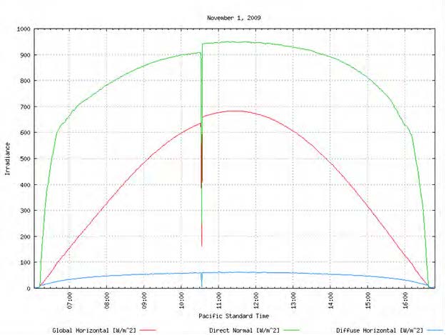
2.4.2.2 Data Quality Assessment
When assimilating a large volume of data, some measure of automated quality assessment must be employed. The methods can range from rudimentary—for example, the temporal behavior of data can be used to identify problems, such as blocked wind vanes or damaged cables; to more sophisticated methods to meet this demand. Depending on how strict the screening parameters are and how their corresponding values are chosen, however, too many or too few events might be detected. A variety of factors—ranging from characteristics of the site and/or instruments to local weather conditions—can affect the data and the validity of screening tests; therefore, the results of the automatic screening always demand a manual check by an expert to ensure their validity. Finally, additional data issues potentially known by the station’s supervisor must be included as comments or flags. Such information should be documented in the metadata (Section 2.4.2.3)

As a general rule, data for inspection should be aggregated to some degree, typically in daily sets (Wilcox and McCormack 2011). This is because individual data points might not lend well to definitive conclusions about quality without the context of many nearby measurements. For example, a sudden change in solar irradiance can often be correlated with the passage of weather fronts that bring clouds and wind. And those conditions might also show a rapid change in temperature, adding to a compelling conclusion.

Data inspection routines should be automated toward the end goal of presenting the quality analyst with on-demand visual plots to streamline the inspection process. This becomes particularly necessary for network operations with dozens of stations where hundreds of thousands of measurements could be generated each day. Background processes can run automated data quality assessment routines and then plot the data and flags in a report readied for the quality analyst to begin inspection. For example, Figure 2-26 holds multiple panels with data graphs from a single station, providing the expert analyst thousands of data points that can be quickly scanned by eye and related with each other to spot inconsistencies.

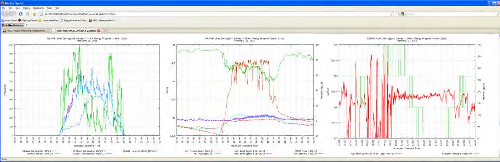
The flags can be visualized next to the data, as shown in Figure 2-27. Here, a suspicious period in the morning was detected by the automatic quality control and marked with the orange background. Of great help is the visualization of the difference between the measured DNI and the DNI calculated from collocated GHI and DHI measurements. This difference plotted over time can help to identify, for example, pyranometer levelling issues, radiometer soiling/dew, or tracking errors.

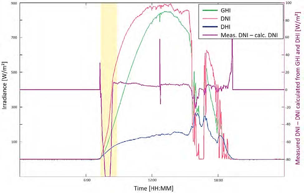
If redundant sensors are used, both measurements or their differences can be plotted and analyzed, which allows for detecting errors that affected only one of the instruments. Digital instruments and some ventilation units for pyranometers also provide additional useful information, such as the rotation speed of the ventilator, the sensor inclination, the sensor acceleration (shock sensor), or error codes. Such data are valuable for quality control and at times allow for corrections before the measurements are strongly affected by the error.

A time series of some measurements can reveal error conditions before they become a problem. Figure 2-28 shows a plot of the daily battery voltage for a remote RSI instrument and indicates a charging problem. In this case, a technician was dispatched, parts were obtained, and the charging circuit was repaired before the instrument lost power and data were lost.

The addition of data quality flags to the data files is an extremely important step in the quality assurance process. For example, the SERI QC software for irradiance measurements (Maxwell, Wilcox, and Rymes 1993) produces flags that can be plotted and included in the rapid visual inspection paradigm (see Figure 2-29). These flags are plotted in the left panel to show a gradation of flag severity from low (dark blue) to high (red) for each minute of a month. To aid the analysis, each solar measurement’s K-space value is plotted in the right three panels, allowing the analyst to find measurement periods that correspond with periods of high flags. Although Figure 2-29 shows a plot for a calendar month, these reports can be generated daily in a moving window to show flagging from previous weeks that lead up to the current day. This allows the analyst to detect error trends early and to formulate a correction.

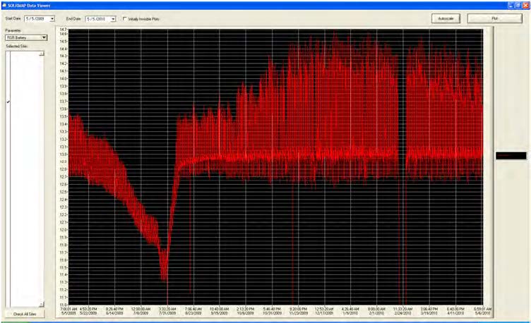
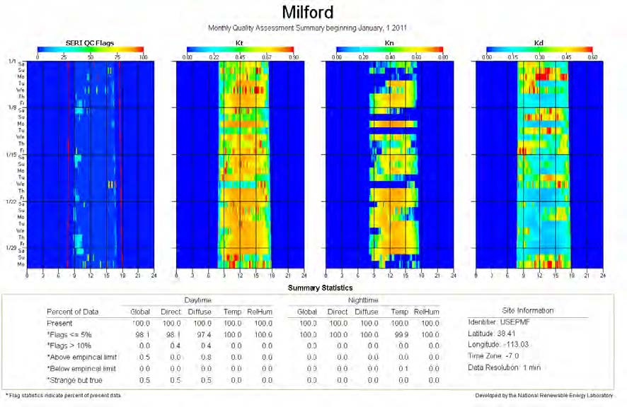
In all these examples, the automated reports should be generated daily (or some other interval consistent with the end use of the data) in preparation for a scheduled session by the analyst, minimizing the amount of manpower required for a thorough data inspection.

Other automated procedures, usually implemented in the data ingest system, employ more rudimentary bounds checking, parameter coupling, and detection of missing data. These checks provide near-real-time triggers for automated email messages to alert operators that a potential error condition exists. These alerts are a first line of defense against serious failures in the system.

2.4.2.3 Metadata and Record-Keeping
The interpretation and application of solar resource measurements depend greatly on the efforts to record and include metadata relevant to the observations. This includes site location; quantitative local horizon surveys with a device visualizing the solar path during the year; data acquisition system(s); input signal channel assignments; radiometer types, models, serial numbers, calibration histories, and installation schemes; and information on eventual post processing of the data and maintenance records. For example, online metadata are available from NREL’s Solar Radiation Research Laboratory.8 Such metadata should be included with the archiving of the measured solar resource data. Examples of issues that need to be documented include damaged or misaligned sensors, maintenance works on the instruments, detection of soiled sensors and subsequent sensor cleaning, obstructed sensors, temporarily erroneous calibration constants in the program code, loose electrical connections, and data logger clock error. These events are frequently not detected automatically or sometimes not even detectable by automatic quality-control screening tools; hence, manual on-site checks are required. The metadata should not necessarily be limited to error conditions and corrections. Information about unusual weather events, animal activity, or even significant flora blooms or vegetation die-off events could prove useful in future analyses that could benefit from knowledge of the measurement environment. Such supplementary information could convey to an auditor that the station operators were thorough in recording station details.

When deciding on a metadata archival method, some consideration should be given to the pros and cons of paper (physical) versus electronic storage. Paper, though not immune to peril, is a simple form that can be read for decades or even centuries. Electronic formats, which are invaluable for easy access and extraction for computer analyses, are too often subject to catastrophic loss through myriad electronic mishaps. Further, changes in the format of once commonplace electronic storage schemes might also render historic metadata unreadable or inaccessible. Using both methods simultaneously solves many of these problems, but it can create new issues with the additional labor for double entry or possible inconsistencies between the two methods.

Figure 2-30 shows a sample paper log that a maintenance technician is required to complete on-site during the maintenance visit. The log not only provides a checklist to ensure a complete inspection but also serves as permanent documentation for the station archive.

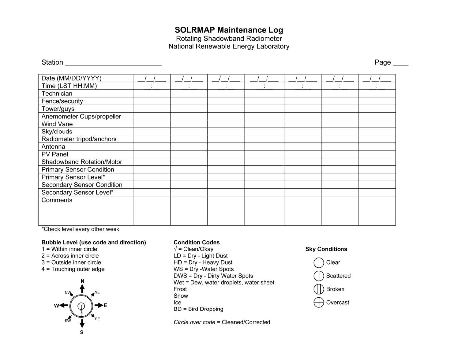
Figure 2-31 shows a (partial) online log form that allows the maintenance technician to remotely access a database interface. Each item in the prescribed maintenance checklist is reported to complete the documentation for the station visit. The log sheet streamlines much of the documentation with codes and checkmarks, and it provides space for freehand comments to describe unusual conditions. For paper logs and online logs, protocols must be in place to ensure that the technician is actually performing the tasks that appear in the logs. At a minimum, station management must be aware of the possibility that a dishonest technician might develop creative ways to falsify a work product. There are ways to remotely verify that the maintenance protocol is being followed. In many cases, when instruments are cleaned, an anomaly appears in the data while the sky irradiance is blocked. The analyst can look at a data plot at the logged time of the visit, and if no disruption appears, further investigation could be warranted. Some systems provide a momentary switch or button that the technician is required to push when arriving on-site. This action places a flag in the data stream verifying that the technician was on-site for the inspection. Remote video cameras can also be a valuable means to verify a proper inspection.

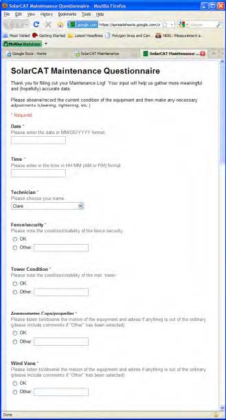
Analysts—whether associated with station operations or employed in a later due diligence process—are immensely aided by ample documentation of station O&M. The documentation, in addition to providing the specific information contained, also indicates the extent of the maintenance protocol. This gives the analyst confidence that problems are discovered and corrected in a minimal amount of time. Further, the documents show that even at well-run stations with a few inevitable malfunctions, best practices and high-quality data govern operations.

Complete documentation includes thorough information in a dedicated metadata archive about the instruments, including manufacturer and model, serial number, calibrations (current and historical), deployment location and configuration, repairs, and inventory or storage details. Of particular importance is the record of instrument calibrations and the associated certificate, traceability, and statement of uncertainty. The calibration record is fundamental to the measurement itself and the assignment of uncertainties to the measured data. Absent a current calibration certificate, a knowledgeable analyst performing validation or due diligence on a data set will likely reject any statement of uncertainty, rendering the measurements highly questionable.

2.4.3 Data Aggregations and Summaries

Solar irradiance measurements for renewable energy applications are becoming more common, and in some electric utility applications, they are required. These measurements are also important for applications in energy-efficiency and climate research. Measurement station design includes data loggers and their configuration as described in Section 2.3.5. Ideally, the station designers will have knowledge in advance about the form (necessary parameters, time resolution, period of record, acceptable uncertainty limits, etc.) of the data required to complete the planned analyses to satisfy the project objectives. But this is not always the case. Further, it is quite common for data sets to be accessed for uses other than their original purpose; thus, the value of a data set could be significantly enhanced if it is in a more generic form that is easily adaptable or convertible to other more specific forms. This typically relates to the frequency of the measurements, which could range from 1 minute to monthly or even yearly.

As noted in Section 2.3.5, the time resolution of the measurements can be increased without significantly increasing the costs for data transfer and storage when compared with the overall costs of operating a station. Because data values can be easily converted to longer timescales, it is recommended that the station be designed to collect data at 1-minute intervals.9 Many commercially available data loggers are capable of sampling the instruments near 1 Hz and then integrating the samples to a 1-minute value (or some other chosen time interval). These values are quite often represented with a unit of W/m2, but the correct unit from this process is W-minute/m2. Most solar analytical tools expect values in Wh/m2, so the conversion must be made prior to further averaging to daily, monthly, or annual values. As a practical matter, the conversion to Wh/m2 can be made by averaging the 1-minute values for 1 hour. The result is mathematically the same as the more descriptively correct method of adding the 60 values in W-minute/m2 and dividing by 60 minutes to convert from the minute to the hourly unit.

Some analytical tools expect hourly values during the period of interest, often a full year. Other tools might expect daily total energy, and others monthly mean daily totals. The conversion from Wh/m2 can then be made to the daily total in Wh/m2 per day by simply adding the hourly values from a single day. From there, the conversion to monthly mean daily totals is accomplished by averaging the daily totals for the month. Examples of reporting monthly solar irradiance measurements are available from https://midcdmz.nrel.gov/apps/report.pl?site=BMS.

In addition to the statistics described, some applications (power plant load matching or building design) look for long-term values by hour of day, for example, the average energy available throughout a month at 11:00. These slices are formed by sorting the hourly data by time stamp and then averaging the subsets during the desired period.

Aggregating solar irradiance and meteorological measurements over various timescales also requires careful attention to methods for estimating the associated measurement uncertainties.

Modeling Solar Radiation: Current Practices

3.1 Introduction

High-quality solar resource assessment accelerates technology deployment by making a positive impact on decision making and by reducing uncertainty in investment decisions. Global horizontal irradiance (GHI), global tilted irradiance (GTI), and/or direct normal irradiance (DNI) are the quantities of interest for solar resource assessment and characterization at a particular location. Surface-based measurements of DNI and GHI can be made only on a relatively sparse network, given the costs of operation and maintenance. GTI is rarely measured in radiometric networks. Nevertheless, observations from ground networks have been used in conjunction with models to create maps of surface solar radiation (Gueymard 2008a). Another option is to use information from geostationary satellites to estimate GHI and DNI at the surface (Cano et al. 1986; Diabate et al. 1988; Pinker and Laszlo 1992; Beyer, Costanzo, and Heinemann 1996; Perez et al. 2002; Rigollier et al. 2004; Cebecauer and Suri 2010; Qu et al. 2016). Because different geostationary satellites are available at different longitudes around the world, radiation can be available for the entire globe (at least between latitudes from approximately -60° to +60°) at temporal and spatial resolutions representative of a particular satellite. For northern and southern high latitudes, a compilation of satellite-derived data based on observations from polar orbiters offers good spatial coverage but typically at a lower spatiotemporal resolution (Karlsson et al. 2017a, 2017b; Kato et al. 2018).

Solar radiation models that use only ground-measured input parameters were used in the past when satellite or weather-model-derived databases were not available. Examples of such models are briefly mentioned for historic reasons. One popular historic model type is based on data from the Campbell-Stokes sunshine duration recorder. The monthly mean GHI is derived using a regression fit to the number of sunshine hours measured by the sunshine recorder’s burn marks when direct solar irradiance exceeds a threshold value of ≈120 W/m2. The regression coefficients are calculated using existing GHI measurements at specific locations. The exact method to calculate GHI using sunshine recorder information is empirical and therefore specific to each geographic area. Moreover, the meteorological services of some countries, such as the United States and Canada, have stopped measuring sunshine duration because of the limited quality and significance of this measurement, which is not standardized and varies from one country to another.

In the absence of surface radiation measurements, estimates of surface radiation can be made using routine meteorological ground measurements and human observations of cloud cover in a radiative transfer model (Marion and Wilcox 1994). For instance, the METeorolgoical-STATistical (METSTAT) model (Maxwell 1998) used information about cloud cover, water vapor, ozone, and aerosol optical depth (AOD) to develop empirical correlations to compute atmospheric transmittance extinction during both clear- and cloudy-sky conditions. That model was used to create earlier versions of the U.S. National Solar Radiation Database (NSRDB) (1991–2005) (e.g., George et al. [2007]). Similar developments have been carried out in Europe with successive versions of the European Solar Radiation Atlas (Page, Albuisson, and Wald 2001).

Long-term GHI data can also be obtained from various numerical weather prediction (NWP) models, either by operating them in reanalysis mode or from actual operational weather forecasts. Examples of reanalysis data include the ERA5 (Hersbach et al. 2019; Trolliet et al, 2018) from the European Center for Medium-Range Weather Forecasting (ECMWF) and the Modern Era Retrospective analysis for Research and Applications, Version 2 (MERRA-2) from the National Aeronautics and Space Administration (NASA) (Bosilovich, Lucchesi, and Suarez 2016; Trolliet et al. 2018). Weather forecasts such as those from the ECMWF’s Integrated Forecasting System (IFS) and the National Oceanic and Atmospheric Administration’s

(NOAA’s) Global Forecast System (GFS) can also provide estimates of GHI. Such estimates, however, are typically not as accurate as those derived from satellite-based models, and they require careful bias corrections (Boilley and Wald 2015, Urraca et al, 2018).
This chapter contains an introduction to satellite-based models, information about currently operational models that provide surface radiation data for current or recent periods, a summary of radiative transfer models used in the operational models, and a discussion of uncertainty in solar-based resource assessments. A short discussion on NWP-based solar radiation data is also included.

3.2 Estimating the Direct and Diffuse Components from Global Horizontal Irradiance 

During clear and partly cloudy conditions, diffuse irradiance on a horizontal surface, DHI, is often only a relatively small part (<30%) of GHI. During dense overcast conditions, GHI and DHI should be identical. When no simultaneous DHI or DNI measurements exist and no alternate determinations are available—for example, from physical-based satellite-based models—DNI and DHI must be estimated from GHI data. Many models based on empirical correlations between GHI and either DHI or DNI data have been developed since Liu and Jordan (1960); Erbs, Klein, and Duffie (1982); Maxwell (1987); Perez et al. (1990); and Louche et al. (1991). More recently, Engerer (2015), Gueymard and Ruiz-Arias (2016), Aler et al. (2017), and Yang and Gueymard (2020) extended this empirical methodology to obtain DNI and DHI at a 1-minute resolution. These algorithms use empirical correlations between the global clearness index, Kt = GHI/[ETR cos(SZA)], and the diffuse fraction, K = DHI/GHI, the diffuse clearness index (i.e., the diffuse transmittance), Kd = DHI/[ETR cos(SZA)], or the direct clearness index (direct transmittance), Kn = DNI/ETR. All these separation models are derived empirically. There are reviews of substantial literature on this topic (e.g., see Gueymard [2008a], Gueymard and Ruiz-Arias [2016], and Tapakis et al. [2016]). Analysts should note that some hourly separation models, including the most popular ones, might not perform correctly if used with subhourly data (Gueymard and Ruiz-Arias 2016).

3.3 Estimating Irradiance on a Tilted Surface

Solar conversion systems, such as flat-plate collectors or non-concentrating photovoltaics (PV), are tilted toward the equator to increase their solar resource. Estimating or modeling the irradiance incident upon them is essential to predicting their performance and yield. This irradiance incident on the plane of array (POA) is usually called GTI, or sometimes simply POA. GTI can be measured directly by pyranometers that are tilted the same as the collector plane. Modeling GTI mainly requires data of the three main components on the horizontal surface

(GHI, DNI, and DHI). GTI can be estimated as the sum of the incident beam, incident sky diffuse, and incident ground-reflected irradiances on the tilted surface; see Eq. 2-2b. The incident beam contribution is simply a straightforward geometric transformation of DNI, requiring only the angle of incidence of DNI on the tilted plane. The ground-reflected contribution is generally small for tilts less than 45°, unless the ground is covered with snow. A simple estimation is possible but requires several assumptions: the foreground is assumed infinite, horizontal, and of isotropic reflectance. In practice, however, the reflected irradiance incident on PV panels outside of the front row would be overestimated with this approach.

The main difficulty is the computation of the sky diffuse irradiance, which has been studied by many authors with different approaches ranging from the simplest isotropic model to more elaborate and complex formulations (Gueymard 1987; Kambezidis, Psiloglou, and Gueymard 1994; Khalil and Shaffie 2013; Liu and Jordan 1960; Loutzenhiser et al. 2007; Muneer and Saluja 1985; Olmo et al. 1999; Padovan and Del Col 2010; Ridley, Boland, and Lauret 2010; Wattan and Janjai 2016; Xie et al. 2016). See the recent review of these models in Yang (2016). Based on the existing studies of the literature, one of the most widely used and validated models is the Perez model (Perez et al. 1987, 1988, 1990). It is the result of a detailed analysis of the isotropic diffuse, circumsolar, and horizon brightening irradiances that are computed by using empirically derived parameters. This approach works well with hourly data, but recently it has been found to generate erroneous values with subhourly data when Kt >1 (i.e., under cloud-enhancement conditions) (Gueymard 2017).

3.4 Introduction to Satellite-Based Models

The goal of satellite-based irradiance models is to use observed information about top-of-atmosphere (TOA) upwelling radiances and atmospheric and surface albedos to derive GHI and DNI at the surface of the Earth. During the last decades, satellite-based retrievals of GHI have been used, for example, for climate studies (Justus et al. 1986). A broad overview of these methods was published by Renné et al. (1999). These methods were originally divided into subjective, empirical/statistical, empirical/physical, and physical methods (Pinker, Frouin, and Li 1995; Schmetz 1989; Myers 2013). The empirical/statistical methods are based on developing relationships between satellite- and ground-based observations; the empirical/physical and theoretical methods estimate surface radiation directly from satellite information using retrieval schemes to determine the atmospheric properties important to radiative transfer. Most empirical/statistical and empirical/physical models are now classified as semiempirical because they involve the development of intermediate relationships either to relate satellite observations with surface radiation measurements or to convert satellite observations directly to solar radiation estimates. Empirical and semiempirical methods generally produce only GHI and require additional models (see Sections 3.2 and 3.4.3) to calculate DNI from GHI. Physical models, on the other hand, generally follow a two-step process that derives cloud optical properties using the satellite radiances in the first step and then computes GHI and DNI using these cloud properties in a radiative transfer model in the second step.

3.4.1 Geostationary Satellites

Geostationary satellites located above the equator that orbit at the same rate as the Earth’s rotation provide continuous coverage of their field of view. Observations are usable up to latitudes 60° N and 60° S because of the Earth’s curvature, as shown in Figure 4-1. The current Geostationary Operational Environmental Satellite (GOES) series covers North and South America (full disk) every 10–15 minutes and the Northern Hemisphere every 5 minutes. Two GOES satellites (GOES-East/GOES-16 and GOES-West/GOES-17) operate concurrently and provide 5-minute coverage for the entire United States. The Advanced Baseline Imager (ABI) on the current GOES satellites makes radiance observations in 16 wavelength bands, or spectral regions (see Table 1) (Schmit et al. 2005; Schmit 2018). GOES-16 became operational in 2018, and GOES-17 became operational in 2019. The wavelengths in Table 1 are representative of the latest generation of geostationary satellite and are similar to those used on the Himawari series of satellites. The previous version of the GOES-East and GOES-West series provided data for five channels (one visible, four infrared) every 30 minutes for the Northern Hemisphere and every 3 hours at full disk.

Table 3-1. GOES-16 and GOES-17 ABI Bands

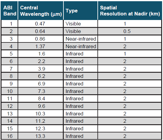
The European Organization for the Exploitation of Meteorological Satellites (EUMETSAT) owns the Meteosat series of satellites that covers Europe, Africa, Middle East, the Indian Ocean, and western Asia. The visible and infrared imager on the Meteosat First Generation (MFG) satellites (up to Meteosat-7) had three visible channels, water vapor (6.2 µm), and infrared. The visible channel produced a 5-km nadir resolution; the infrared channel’s nadir resolution was also 5 km. Moreover, there were two channels with 2.5-km resolution, in interleaved format. Imagery had a repetition frequency of 30 minutes. The Spinning Enhanced Visible and InfraRed Imager (SEVIRI) on the Meteosat Second Generation (MSG) satellites (Meteosat-8 onward) provides satellite imagery every 15 minutes at a nominal 3-km resolution for 11 channels (Schmetz et al. 2002). The 12th channel, a high-resolution visible channel, has a nadir resolution of 1 km.

The Himawari-8 is a third-generation satellite similar to GOES-16 and the EUMETSAT’s Meteosat Third Generation (MTG) satellites and covers East Asia and the Western Pacific. Himawari-8 was launched in October 2014 and harbors the Advanced Himawari Imager, which has characteristics similar to the ABI (Besho et al. 2016). Of the 16 bands, the visible and near-infrared bands measure resolutions at 0.5 km or 1 km, whereas the infrared bands measure at 2 km. A full-disk image is produced every 10 minutes, and the sectors are generated every 2.5 minutes. Himawari-8 replaced the Multifunctional Transport Satellite series of satellites, which had been in operation since 2005.

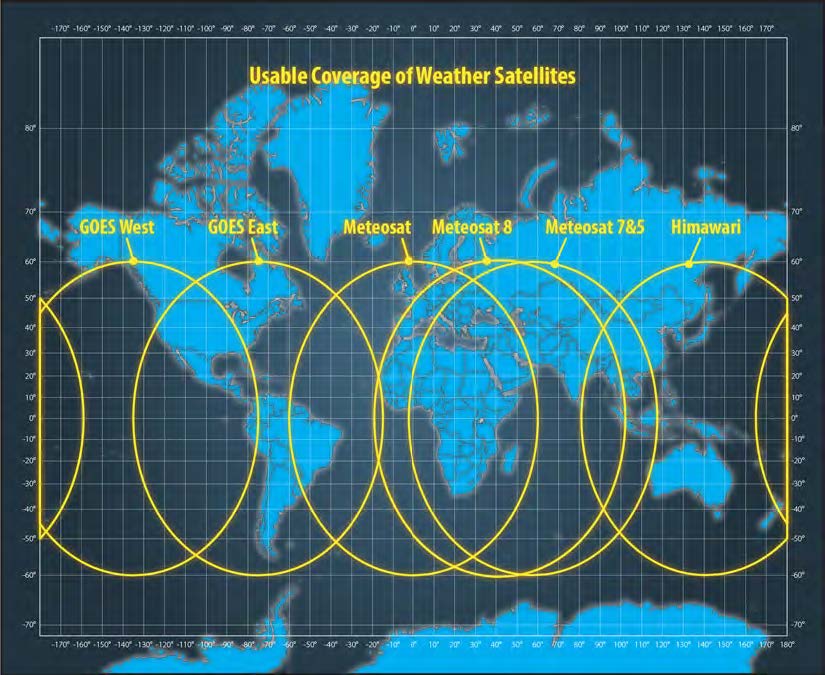
3.4.2 Polar-Orbiting Satellites

Polar-orbiting satellites are used to continuously sense the Earth and retrieve cloud properties and solar radiation at the surface. An example of one such instrument is the Advanced Very High Resolution Radiometer (AVHRR) on the NOAA series of polar-orbiting platforms. Other examples are the Moderate Resolution Imaging Spectroradiometer (MODIS) and the Clouds and the Earth’s Radiant Energy System (CERES) instruments on NASA’s Aqua and Terra satellites. The Joint Polar Satellite System (JPSS) series of satellites is expected to replace the legacy NOAA polar satellites. The first satellite in the JPSS series was launched in 2011 and is called the Suomi National Polar-Orbiting Partnership. The second satellite, NOAA-20, was launched in 2017. This next-generation series of satellites has multiple instruments, including the Visible Infrared Imaging Radiometer Suite, Cross-track Infrared Sounder, Advance Technology Microwave Sounder, Ozone Mapping and Profiler Suite, and CERES. Although polar orbiters provide global coverage, their temporal coverage is limited because of their orbit, in which they essentially cover a particular location only once per day at the lower latitudes. At higher latitudes, a combination of many polar-orbiting, satellite-based products is recommended to achieve a sufficient temporal resolution while also benefiting from better spatial resolution.

3.4.3 Satellite-Based Empirical and Semiempirical Methods

Satellite-based semiempirical methods consider a pseudo-linear correlation between the atmospheric transmittance and the radiance sensed by the satellite. Semiempirical models are classified as such because of their hybrid approach to retrieving surface radiation from satellite observations, in which the normalized satellite-observed reflectance is related to GHI at the surface. Cloud-cover indices that use visible satellite imagery are first created with budget equations between TOA and surface radiation. Those indices are then used to modify the clear-sky GHI and estimate GHI at the ground consistent with the cloud scene. DNI can then be derived from GHI and the clear-sky DNI using one of the empirical methods discussed later in this subsection. The semiempirical approach was originally designed to create regression relationships between what is simultaneously observed by a satellite and ground-based instruments (Cano et al. 1986; Hay et al. 1978; Justus et al. 1986; Tarpley 1979). The method developed by Cano et al. (1986) is called the Heliosat method. It has been regularly updated and modified to rely on atmospheric transmittance properties of water vapor and aerosols to provide solar radiation estimates under clear-sky conditions rather than direct empirical relationships with ground data.

The original Heliosat method evaluates the clearness index, Kt, or the ratio of the radiative flux at the Earth’s surface and the radiative flux at the TOA (which is known), using the relationship:

where a and b are the slope and intercept of the assumed linear relation, and n is the so-called cloud index defined as:

where ρ , ρ cloud, and ρ g are the satellite-based reflectance observations of the current scene, of the brightest clouds, and of the ground, respectively. The cloud index is close to 0 when the observed reflectance is close to the ground reflectance (i.e., when the sky is clear). It can be negative if the sky is very clear, in which case ρ is smaller than ρ . The cloud index increases as clouds appear, and it can be greater than 1 for clouds that are optically very thick.

The parameters a and b in Eq. 3-1 can be derived empirically by comparison with coincident ground measurements or they can determined based on the physical principles of atmospheric transmittance, which include not only the cloud index but also the influence of aerosols, water vapor, and trace gases. Diabate et al. (1988) observed that three sets of parameters for the morning, noon, and afternoon were needed for Europe. The Heliosat method (and all cloud-index-based methods) requires the determination of cloud-free and extremely high cloud reflectivity instances to establish bounds to Eq. 3-1. Espinar et al. (2009) and Lefèvre, Wald, and Diabate (2007) found that a relative error in the ground albedo related to errors in determining the reflectivity from a cloud-free pixel leads to a relative error of the same magnitude in GHI under clear-sky conditions, which corresponds to approximately 10% of the GHI in clear cases. In cloudy cases, the error, which is caused by an error in the limit for the albedo of the brightest clouds, increases as cloud optical depth (COD) increases, and the relative error in the GHI can reach 60% (Espinar et al. 2009; Lefèvre, Wald, and Diabate 2007).

Beyer, Costanzo, and Heinemann (1996) developed an enhanced version of the Heliosat method called Heliosat-1. One major enhancement was the adoption of the clear-sky index, Kc (the ratio of the actual GHI to the GHI under ideal clear conditions), instead of the clearness index, Kt. This resulted in the relationship Kc = 1 – n, which simplified the method. Additional work was done to remove the dependence of the satellite radiance based on the sun-to-satellite geometry, thereby leading to a more spatially homogeneous cloud index. In addition, the determination of ground albedo and cloud albedo was improved by Beyer, Costanzo, and Heinemann (1996). Rigollier et al. (2004) developed Heliosat-2, which further enhanced Heliosat-1 by removing parameters that needed to be tuned and replacing them with either constants or values that can be computed automatically during the process. The HelioClim-3 and Solar Energy Mining
(SOLEMI) databases, produced by MINES ParisTech and DLR, respectively, use Heliosat-2. The Heliosat-3 version was designed collaboratively by the University of Oldenburg, MINES ParisTech, and DLR, among others, and it uses the SOLIS clear-sky model, which approximates radiative transfer equations for fast implementation (Müller et al. 2004). Centro de Investigaciones Energéticas, Medioambientales y Tecnológicas (CIEMAT) and its spin-off, IrSoLaV, performed remarkable modifications on the Heliosat-3 scheme. This resulted in a different model, which includes a clear-sky detection algorithm, different possible clear-sky models with atmospheric component data sets as input, and a dynamic model for estimating the ground albedo as a function of the scattering angle (Polo et al. 2012, 2013).

Hay et al. (1978) developed a regression model that relates the atmospheric transmittance to the ratio of incoming to outgoing radiation at the TOA. The transmittance was then used to derive GHI. In this method, the coefficients of the regression model change significantly based on location, and they need to be trained with surface observations (Nunez 1990) to produce accurate results. The Tarpley (1979) method also used the well-known relation between surface radiation, TOA radiation (both upwelling and downwelling), and atmospheric transmittance to create three separate regression equations. The regression equations were classified based on sky conditions labeled as clear, partly cloudy, and cloudy, and they were used accordingly.

Models such as those developed by Perez et al. (2002), Rigollier et al. (2004), and Cebecauer and Suri (2010) evolved from Cano et al. (1986) and included refinements to address albedo issues, when the surface is covered by snow, and the effects of sun-satellite geometry. Some of these models have since been modified to include the simplified SOLIS model (Ineichen 2008), and are used to estimate GHI first and then DNI after component separation (Section 3.2).

3.4.4 Satellite-Based Physical Models

Physical models generally use radiative transfer theory to directly estimate surface radiation based on first principles using cloud properties, water vapor, AOD, and ozone as inputs. The radiative transfer models can be classified as either broadband or spectral, depending on whether the radiative transfer calculations involve a single broadband calculation or multiple calculations in different wavelength bands.

The broadband method of Gautier et al. (1980) used thresholds depending on multiple days of satellite pixel measurements to determine clear and cloudy skies. Separate clear-sky and cloudy-sky models were then used to evaluate the surface DNI and GHI. The clear-sky model initially included water vapor and Rayleigh scattering but progressively added ozone (Diak and Gautier 1983) and aerosols (Gautier and Frouin 1984). Assuming that attenuation caused by the atmosphere does not vary from clear to cloudy conditions, Dedieu, Deschamps, and Kerr (1987) created a method that combines the impacts of clouds and the atmosphere. This method uses a time series of images to determine clear-sky periods for computing surface albedo. Darnell et al. (1988) created a parameterized model to calculate surface radiation using a product of the TOA irradiance, atmospheric transmittance, and cloud transmittance. Developed with data from polar-orbiting satellites, this model used collocated surface and satellite measurements to create relationships between cloud transmittance and planetary albedo.

Möser and Raschke (1983) created a model based on the premise that GHI is related to fractional cloud cover and used it with Meteosat data to estimate solar radiation over Europe (Möser and Raschke 1984). The fractional sky cover was determined to be a function of satellite measurements in the visible channel. This method uses radiative transfer modeling (Kerschgens et al. 1978) to determine the clear- and overcast-sky boundaries. Stuhlmann et al. (1990) have since enhanced the model to include elevation dependence and additional constituents as well as multiple reflections in the all-sky model.

An important spectral model developed by Pinker and Ewing (1985) divided the solar spectrum into 12 intervals and applied the Delta-Eddington approximation for radiative transfer (Joseph et al. 1976) to a three-layer atmosphere. The primary input to the model is the COD, which can be provided from various sources. This model was enhanced by Pinker and Laszlo (1992) and used in conjunction with cloud information from the International Satellite Cloud Climatology Project (ISCCP) (Schiffer and Rossow 1983). Another physical method involves the use of satellite information from multiple channels to derive cloud properties (Stowe et al. 1999) and then evaluate DNI and GHI using the cloud properties in a radiative transfer model. This method, called CLOUDS, was originally developed using the polar-satellite data from the AVHRR instrument onboard NOAA satellites, and the processing system was called Clouds from AVHRR Extended System (CLAVR-x) (Heidinger 2003; Pavolonis et al. 2005). This method has been modified and enhanced to use cloud properties from the GOES satellites (Heidinger 2003; Pavlonis et al. 2005). In 2013, CLAVR-x was updated again to support the generation of higher spatial resolution output for the NOAA National Centers for Environmental Prediction and incorporated many algorithm improvements from the GOES-R Algorithm Working Group effort.

The cloud information produced from the CLAVR-x type of algorithms can then be input to a radiative transfer model, such as the Fast All-sky Radiation Model for Solar applications (FARMS) (Xie et al. 2016), to calculate GHI and DNI, as has been done for the development of the most recent versions of the National Renewable Energy Laboratory’s (NREL’s) gridded NSRDB (1998–2015).

Another cloud retrieval scheme, called AVHRR Processing scheme Over cLouds, Land, and Ocean (APOLLO), was developed by Kriebel et al. (1989, 2003) for the AVHRR instrument. APOLLO has been adapted for use with data obtained from the SEVIRI instrument on the MSG satellite. APOLLO-derived cloud products, including COD and cloud type, can be used in a radiative transfer model such as Heliosat-4 (Oumbe 2009; Qu et al. 2016), made operational by the Copernicus service (http://www.copernicus-atmosphere.eu).
The ISCCP (Schiffer and Rossow 1983) was established in 1982 as part of the World Climate Research Programme. The ISCCP cloud products include COD, cloud top temperature, cloud particle size, and other cloud properties that could be used to derive surface radiation.
Physical models are computationally more intensive than empirical and semiempirical models. Advantage of physical models, however, are that they can use additional channels from new satellites (such as MSG or GOES-16) to improve cloud property retrieval and can include physical properties of aerosols and other gaseous species, such as water vapor, explicitly.

3.5 Clear-Sky Models Used in Operational Models

3.5.1 Bird Clear-Sky Model

The Bird clear-sky model (Bird and Hulstrom 1981) is a broadband algorithm that produces estimates of clear-sky direct beam, hemispherical diffuse, and total hemispherical solar radiation on a horizontal surface. The model uses a parameterization based on radiative transfer computations and comprising simple algebraic expressions. Model results are expected to agree within ±10% with detailed high-resolution spectral or broadband physics-based radiative transfer models. The model can be used at resolutions of 1 minute or better and can duly accept inputs at that frequency, if available. In the absence of high-temporal-resolution input parameters, however, climatological or annual average values can be used alternatively as inputs to the model. The Bird clear-sky model also forms the basis of the clear-sky part of METSTAT, with only minor modifications. The performance of these two models has been assessed rigorously and compared to other algorithms (Badescu et al. 2012; Gueymard 1993, 2003a, 2003b, 2004a, 2004b, 2012; Gueymard and Myers 2008; Gueymard and Ruiz-Arias 2015).

3.5.2 European Solar Radiation Atlas Model

The European Solar Radiation Atlas (ESRA) model is another example of a clear-sky model (Rigollier et al. 2000). Used in the Heliosat-2 model that retrieves GHI from satellites, this model computes DNI, GHI, and DHI using Rayleigh optical depth, elevation, and the Linke turbidity factor as its inputs. The performance of the model has been evaluated at various locations (Badescu et al. 2012; Gueymard and Myers 2008; Gueymard 2012; and Gueymard and Ruiz-Arias 2015).

3.5.3 SOLIS Model

The SOLIS model (Müller et al. 2004) is a relatively simple spectral clear-sky model that can calculate DNI, GHI, and diffuse radiation based on an approximation to the Lambert-Beer relation for computing DNI:

where:

• τ is the atmospheric optical depth at a specific (monochromatic) wavelength
• M is the optical air mass
• I0 is the TOA spectral direct irradiance for a monochromatic wavelength
• I is the DNI at the surface for a monochromatic wavelength.

This equation is modified to account for slant paths and adapted for global and diffuse radiation. The modified Lambert-Beer relation (Müller et al. 2004) is:

where:

• I(SZA) is one of the irradiance components GHI, DNI, or DHI
• c is the empirical exponent that depends on the radiation component DNI, DHI, or GHI
• τc is the vertical broadband optical depth of the atmosphere for the radiation component of interest
• SZA is the solar zenith angle.

The Beer-Lambert equation is a simple relationship because it accounts for monochromatic DNI and is impacted only by atmospheric attenuation. On the other hand, DHI and GHI are broadband values that contain energy that is scattered by the atmosphere. The empirical exponent c is used as an adjustment to compute either GHI or DHI, as explained in Müller et al. (2004). Ineichen (2008) developed a simplified (broadband) version of that clear-sky model by developing parameterizations to replace radiative transfer model runs, thereby increasing the speed of the model.

3.5.4 McClear Model

The fast clear-sky broadband model called McClear implements a fully physical model, replacing the empirical relations or simpler models used before, such as ESRA. It exploits the recent results on aerosol properties and total column content in water vapor and ozone produced by the European Copernicus Atmosphere Monitoring Service (CAMS) project. It is based on lookup tables precomputed with the radiative transfer model libRadtran (Gschwind et al. 2019). McClear irradiances were compared to 1-minute measurements made under clear-sky conditions at several Baseline Surface Radiation Network (BSRN) stations representative of various climates (Lefèvre et al. 2013). For GHI and DNI, the correlation coefficients range from 0.95–0.99 and from 0.86–0.99, respectively. The bias ranges from 14–25 W/m² and 49–33 W/m², respectively. The root mean square errors range from 20 W/m² (3% of the mean observed irradiance) to 36 W/m² (5%) and from 33 W/m² (5%) to 64 W/m² (10%), respectively.

3.5.5 REST2 Model

The high-performance REST2 model is based on transmittance parameterizations over two distinct spectral bands separated at 0.7 µm. The model’s development and its benchmarking are described by Gueymard (2008b). REST2 has been thoroughly validated and compared to other irradiance models under varied atmospheric conditions, including extremely high aerosol loads (Antonanzas-Torres et al. 2016; Engerer and Mills 2015; Gueymard 2012, 2014; Gueymard and Myers 2008; Gueymard and Ruiz-Arias 2015; Sengupta and Gotseff 2013; Zhong and Kleissl 2015).
The model is used in solar-related applications, including the benchmarking of the radiative output of the Weather Research and Forecasting (WRF) model (Ruiz-Arias et al. 2012), the operational derivation of surface irradiance components using MODIS satellite observations
(Chen et al. 2014), the improvement in GHI to DNI separation modeling (Vindel et al. 2013), and the development of future climate scenarios (Fatichi et al. 2011). REST2 is also being used at NREL (Xie et al. 2016) and is integrated into its suite of algorithms that produces the current version of the NSRDB (1998–2019).

3.6 All-Sky Models Used in Operational Models

3.6.1 Fast All-Sky Radiative Transfer Model

Radiative transfer models are capable of simulating atmospheric radiation under all-sky conditions and have been used in a broad range of applications, such as satellite remote sensing or climate studies. Compared to other applications, solar energy has unique requirements from radiative transfer models and thus has particular prerequisites in the model design. For instance, the study of solar energy demands more efficient simulations of solar irradiance than the conventional models used in weather or climate studies, such as the Rapid Radiation Transfer Model (RRTM) or its simplified two-stream version for inclusion in general circulation models (RRTMG). To provide a new option for efficiently computing solar radiation, NREL developed FARMS (Xie et al. 2016) using cloud transmittances and reflectances for direct and diffuse radiation computed by RRTM with the 16-stream discrete-ordinates radiative transfer method. To reduce the computing burden, the cloud transmittances and reflectances are parameterized as functions of SZA, cloud thermodynamic phase, optical thickness, and particle size. The all-sky GHI, DHI, and DNI are ultimately computed by coupling the cloud transmittances and reflectances with surface albedo and a fast clear-sky radiation model (REST2) to account for atmospheric absorption and scattering.

To understand the accuracy and efficiency of FARMS, GHI was simulated using the cloud microphysical and optical properties retrieved from GOES data during 2009–2012 with both FARMS and RRTMG and compared to measurements taken at the Southern Great Plains site of the U.S. Department of Energy’s Atmospheric Radiation Measurement Climate Research Facility. Results indicate that the accuracy of FARMS is comparable to, if not better than, the two-stream approach; however, FARMS is approximately 1000 times more efficient and faster because it does not explicitly solve the radiative transfer equation for each individual cloud condition.

Note that FARMS, as well as the conventional radiative transfer models developed for weather and climate studies, outputs only broadband irradiance over horizontal surfaces. Recently, FARMS expanded its capabilities to incorporate tilted surfaces and spectral distributions (Xie and Sengupta 2018; Xie, Sengupta, and Wang 2019).

3.6.2 All-Sky Models Used in the Recent Heliosat Model

The CAMS radiation service uses a physical retrieval of cloud parameters and the fast parameterized radiative transfer method called Heliosat-4 (Qu et al. 2016). The new Heliosat-4 method computes GHI, DNI, and DHI under all-sky conditions as a broadband aggregation of spectrally resolved internal computations. It is a fast but accurate physical model that mimics a full radiative transfer model, and it is well suited for geostationary satellite retrievals. The method is based on the work of Oumbe et al. (2014), which proved that the surface solar irradiance can be approximated by the product of the irradiance under cloudless conditions and a modification index depending only on cloud properties and ground albedo. This is why Heliosat-4 contains two precomputed lookup-table-based models: the McClear model (Lefèvre et al. 2013; Gschwind et al. 2019) for clear-sky conditions and the McCloud model for cloudy conditions. The databases for both models were developed using the libRadtran radiative transfer model (Mayer and Kylling 2005). The main inputs to McClear are aerosol properties, total column water vapor, and ozone, whereas cloud properties, such as COD, are the main inputs to the McCloud part of Heliosat-4. With MSG satellite observations, cloud properties are derived at a 15-minute temporal resolution using an adapted APOLLO retrieval scheme. An easy-to-read summary can be found in the “User’s Guide to the CAMS Radiation Service”10 (Schroedter-Homscheidt et. al. 2016).

3.6.3 Cloud Physical Properties-Surface Insolation under Clear and Cloudy Skies Algorithm

The Cloud Physical Properties (CPP) retrieval algorithms have been developed in EUMETSAT’s Satellite Application Facility on Climate Monitoring (CM SAF)11 as well as other European and national (The Netherlands) projects (Roebeling et al. 2006; Stengel et al. 2014; Karlsson et al. 2017a, 2017b; Benas et al. 2017). The basic retrieved parameters are cloud mask, cloud-top height, cloud thermodynamic phase, COD, particle effective radius, and water path. From these parameters, surface downwelling shortwave radiation is derived, as well as precipitation.

The CPP algorithm first identifies cloudy and cloud-contaminated pixels using a series of thresholds and spatial coherence tests imposed on the measured visible and infrared radiances (Roebeling et al. 2006; 2009). Depending on the tests, the sky can be classified as clear, contaminated, or overcast. Subsequently, cloud optical properties (COD and effective radius) are retrieved by matching observed reflectances at visible (0.6 μm) and near-infrared (1.6 μm) wavelengths to simulated reflectances of homogeneous clouds comprising either liquid or ice particles. The thermodynamic phase (liquid or ice) is determined as part of this procedure using a cloud-top temperature estimate as additional input.

Building on the retrieval of cloud physical properties, the Surface Insolation under Clear and Cloudy Skies (SICCS) algorithm was developed to estimate surface downwelling solar radiation using broadband radiative transfer simulations (Deneke et al. 2008; Greuell et al. 2013). GHI, DNI, and DHI are retrieved. The cloud properties are the main input for cloudy and cloud-contaminated (partly cloudy) pixels. Information about atmospheric aerosol from the Monitoring Atmospheric Composition and Climate (MACC) is used for cloud-free scenes. Other inputs for the CPP and SICCS algorithms include surface elevation from the ETOPO2v2-2006 database, monthly varying integrated atmospheric water vapor from the ECMWF ERA-Interim reanalysis, and 8-day varying surface albedo derived from MODIS data.

3.7 Numerical Weather Prediction-Based Solar Radiation Estimates

NWP models, run either in reanalysis mode or to generate weather forecasts, can provide GHI estimates for long periods of time. The accuracy of such estimates is known to be less than those provided by satellite-based models. Significant improvements, however, can be obtained by improving both the model physics and the assimilation of various observations. Some commonly available models and data sets are described in the following sections. Note that this is not a complete and comprehensive list. The goal is only to provide the user with initial information related to this potential source of data.

3.7.1 Reanalysis Models

ERA5 is a global atmospheric reanalysis that provides data starting in 1979. This data set is produced using the ECMWF’s data assimilation system used in the IFS. This system uses four-dimensional variational analysis and provides analysis data with TOA and both GHI and direct horizontal irradiance (all-sky and clear-sky) in hourly time resolution on an approximate 0.25° x 0.25° grid. More information can be found on the Copernicus ERA5 website.12

NASA’s MERRA-2 is another global atmospheric reanalysis data set that provides data starting in 1980 and comprises TOA and GHI (all-sky and clear-sky). It includes additional data sets from those assimilated into the original MERRA data set. The spatial resolution is 0.5° x 0.625°, and the temporal resolution is hourly.13

Finally, the Climate Forecast System Reanalysis from NOAA provides reanalysis data from 1979. The GHI data are available hourly at a 0.5° resolution.14

3.7.2 Forecast Models

Various national meteorological agencies run operational weather forecasts both regionally and globally. Some data from these operational models might be available from archives. Some of the most popular examples of global data sets are from the ECMWF’s IFS runs and from NOAA’s GFS runs. There are various regional model runs by national meteorological agencies that produce forecasts for individual countries and regions. Because many data sets now exist, this type of data is mentioned without pointing to specific sources.

Solar forecasting requires improved forecasting of clouds, which is generally a weakness in many NWP models, so there have been significant recent efforts to improve cloud and radiation modeling, especially within the WRF mesoscale model. This led to the development of the WRF-Solar model (Jimenez et al. 2016), which includes significant improvements in cloud modeling as well as the capability to compute surface radiation using FARMS.

3.8 Site Adaptation: Merging Measurements and Models

A major goal of solar resource assessments is to provide high-quality data to evaluate the financial viability of solar power plant projects (Moser et al., 2020). This essentially implies that accurate data over long time periods are available for conducting these studies. Normally, satellite-derived data time series fulfill the requirement for long-term data; however, they could be hampered by inherent biases and uncertainty because of the following:

• The information content, quality, and spatial and temporal resolution of the raw satellite data
• The approximations made by the models converting satellite observations into surface solar radiation estimates
• The uncertainty in ancillary information needed by these models
• The empirical process used to separate the direct and diffuse components.

As part of a resource assessment study for a new large solar power plant, ground-based solar measurements are conducted for a short period of time (nominally approximately 1 year) and used to validate the satellite data. The main goal is to remove some of the uncertainties and bias in modeled data sets. This process has been given various names, including “site adaptation,” which is used here for simplification. A review paper by Polo et al. (2016) provides a summary of the various methods currently used.

Note, however, that the ground-based irradiance data need to be of high quality, otherwise the correction method could degrade the quality of the modeled time series. High-quality ground measurements can be achieved only by using well-calibrated, high-quality instruments that have been deployed at well-chosen locations using optimal installation methods and regular maintenance, per the best practices described in other sections.

Site-adaptation methods can be separated into two broad categories. The first consists of physical methods that attempt to reduce the uncertainty and bias in the data by improving the satellite model inputs, such as AOD. The second approach develops statistical correction schemes directly comparing the satellite-based irradiance estimates with “unbiased” ground observations and uses those functions to correct the satellite-based radiation estimates.

Various site-adaptation methods have been benchmarked (Polo et al., 2020) within the International Energy Agency’s Photovoltaic Power Systems Programme Task 16. In that study, 11 different site-adaptation techniques have been used to assess improvements in accuracy. Ten different data sets covering both satellite-derived and reanalysis solar radiation data were used. The effectiveness of these methods is not found to be universal or spatially homogeneous, but in general it can be stated that significant improvements can be achieved eventually for most sites and data sets.

3.8.1 Physical Methods

Because the highest uncertainty in satellite models is in DNI, the primary goal is to reduce errors in DNI by improving the quantification of AOD. Methods such as those proposed by Gueymard (2011, 2012) demonstrate how accurate AOD data obtained from ground sunphotometric measurements can indeed improve DNI. Nevertheless, the scarcity of such high-quality AOD observations implies that other sources should be used. Possible sources of AOD with global coverage include retrievals from the MODIS and MISR satellites, data assimilation output from CAMS, and NASA’s MERRA-2 data (Gueymard and Yang 2020). In parallel, specific methods have been developed by Gueymard and Thevenard (2009) and Ruiz-Arias et al. (2013a, 2013b) to correct biases and uncertainties in the satellite- or model-based AOD data using ground observations. These adjusted AOD data sets have been shown to improve the satellite-based solar radiation estimates at various locations.

3.8.2 Statistical Methods

Various statistical methods have been developed to use short-term ground measurements to directly correct long-term satellite-based data sets. These bias correction methods range from linear methods (Cebecauer and Suri 2010; Vindel et al. 2013; Harmsen et al. 2014; Polo et al. 2015) to various nonlinear methods, including feature transformation (Schumann et al. 2011), polynomial-based corrections (Mieslinger et al. 2014), model output statistics corrections (Bender et al. 2011; Gueymard et al. 2012), measure-correlate-predict corrections (Thuman et al. 2012), and Fourier-decomposition-based corrections (Vernay et al. 2013). Other statistical methods include regional fusion methods of ground observations with satellite-based data (Journée et al. 2012; Ruiz-Arias et al. 2015) and improvements to the irradiance cumulative distribution function (Cebecauer and Suri 2012; Blanc et al. 2012).

3.9 Summary

This chapter provided a brief overview of solar radiation modeling methods with a focus on satellite-based models. Since the 1980s, both the technology of operational meteorological satellites and models to estimate surface radiation from these satellites have improved in their resolution and accuracy. With the recent launch of GOES-16, the world is now mostly covered at temporal resolutions of 15 minutes or better and spatial resolutions of 1 km. Improvements in computational capabilities have also contributed to improving our ability to use increasingly sophisticated models that can use higher volumes of satellite and ancillary data sets and ultimately deliver products of increasing resolution and accuracy.

This chapter also contained a short introduction to NWP modeling because improvements in that area can contribute to better irradiance estimates around the globe. This chapter has been kept deliberately short while providing the interested readers with references for more detailed reading. Finally, the following appendix provides short descriptions of some commonly used satellite-based data sets.

Appendix: Currently Available Satellite-Based Data Sets

This section presents examples of currently available operational models. Only a selection of models is presented here. Further public, scientific, and commercial operational models exist and might also be of interest for solar resource analyses.

National Solar Radiation Database Physical Solar Model (2019 Update)

For many years, the National Renewable Energy Laboratory (NREL) has maintained a ground-based solar radiation data set known as the National Solar Radiation Database (NSRDB). This data set included both actual in situ ground measurements and the METeorolgoical-STATistical model (METSTAT) model (Maxwell et al. 1997) to convert U.S. National Weather Surface ground-based sky observations to solar radiation estimates. The original NSRDB (1961–1990) (NREL 1992) covered the period from 1961–1990 for 239 ground stations in the United States. That original version of the NSRDB was subsequently updated to cover an extended period
(1991–2005), including many more ground stations and making use of satellite-based data to correct for some ground-based measurements (NREL 2007).

In collaboration with the University of Wisconsin and the National Oceanic and Atmospheric Administration, NREL produced a physics-based satellite-derived solar radiation data set as part of a new gridded NSRDB (1998–2019) (Xie and Sengupta 2018). This gridded NSRDB (1998–2019) uses the Physical Solar Model (PSM), which produces satellite-based data every 30 minutes for 4-km-resolution pixels for North American and South America and is freely available from the NSRDB website (https://nsrdb.nrel.gov). The data fields include solar radiation and meteorological data. With the availability of the next-generation Geostationary Operational Environmental Satellites (GOES-16 and GOES-17), the NSRDB is currently producing 5-minute data for most of the Northern Hemisphere and 10- to 15-minute data for both the Northern Hemisphere and Southern Hemisphere. These data are being produced at a 2-km spatial resolution.

The PSM (currently Version 3) consists of a two-stage scheme that retrieves cloud properties and uses those properties in a radiative transfer model to compute surface radiation. In the first stage, cloud properties are generated using the Advanced Very High Resolution Radiometer (AVHRR) Pathfinder Atmospheres-Extended (PATMOS-x) algorithms (Heidinger et al. 2014). In the second stage, global horizontal irradiance (GHI) and diffuse horizontal irradiance (DHI) are computed by the Fast All-sky Radiation Model for Solar applications (FARMS) model (Xie et al. 2016) using these cloud properties as well as additional meteorological parameters as inputs. The FARMS model uses the REST2 model (Section 3.5.5) for clear-sky calculations and a fast all-sky model for cloudy-sky calculations (Section 3.6.1). The aerosol optical depth (AOD) inputs required for clear-sky calculations are obtained from the hourly Modern Era Retrospective analysis for Research and Applications, Version 2 (MERRA-2) aerosol products from the National Aeronautics and Space Administration (NASA) after scaling and bias reduction using ground AOD measurements from the Aerosol Robotic Network (AERONET). Water vapor, temperature, wind speed, relative humidity, and dew point data are obtained from NASA’s MERRA-2.

The NSRDB also provides spectral data sets for 2002 wavelengths. The spectral data are produced on demand and use the FARMS-Narrowband Irradiance on Tilted Surface (FARMS-NIT) model (Xie and Sengupta 2018; Xie et. al. 2019).

The time-series irradiance data for each pixel are quality-checked to ensure that they are within acceptable physical limits, that gaps are filled, and that the Coordinate Universal Time stamp is shifted to local standard time. Finally, the GOES-East and GOES-West data sets are blended to create a contiguous data set for the period from 1998–2019.

National Aeronautics and Space Administration/Global Energy and Water Cycle Experiment Surface Radiation Budget

To serve the needs of the World Climate Research Program, Whitlock et al. (1995) developed a global Surface Radiation Budget (SRB) data set using cloud information from the International Satellite Cloud Climatology Project (ISCCP) C1 data set at a resolution of 250 km by 250 km (approximately 2.5° x 2.5°) every 3 hours (Schiffer and Rossow 1983; Zhang et al. 2004). Information from the ISCCP C1 data set is used as an input into the Pinker and Laszlo (1992) model and the Darnell et al. (1988) model.

The currently available version is the NASA/Global Energy and Water Cycle Experiment SRB Release 3.0 data set that contains global 3-hour, daily, monthly/3-hour, and monthly averages of surface longwave and shortwave radiative parameters on a 1° x 1° grid. Primary inputs to the models include:

• Visible and infrared radiances and cloud and surface properties inferred from ISCCP pixel-level data
• Temperature and moisture profiles from the GEOS-4 reanalysis product obtained from NASA’s Global Modeling and Assimilation Office
• Column ozone amounts constituted by assimilating various observations.

The SRB data set is available from multiple sources. The Surface meteorology and Solar Energy (SSE) website provided SRB data in a version that was more applicable to renewable energy. SSE has recently been replaced by an improved version called POWER.15 SRB data sets are also available from the Clouds and the Earth’s Radiant Energy System (CERES) project.16 Additionally, the Fast Longwave and Shortwave Radiative Fluxes (FLASHFlux) project generates real-time SRB data.17 All these projects use global observations from CERES and Moderate Resolution Imaging Spectroradiometer (MODIS) instruments onboard polar-orbiting satellites. Table 4-2 shows the estimated bias and root-mean-square (RMS) error between the original NASA SSE irradiation estimates and measured World Meteorological Organization

(WMO) Baseline Surface Radiation Network (BSRN) monthly averages of the three usual solar radiation components. The NASA POWER accuracy and methodology are documented on its website.

Table 3-2. Regression Analysis of NASA SSE Compared to BSRN Bias and RMS Error for Monthly Averaged Values from July 1983–June 2006

German Aerospace Center (DLR)-Irradiance at the Surface Derived from ISCCP Cloud Data (ISIS) Model (DLR-ISIS Model)

Similar to the NASA SSE and POWER data sets, the DLR-ISIS data set18 is a 21-year direct normal irradiance (DNI) and GHI data set based on the ISCCP cloud product covering the period from July 1983–December 2004. The cloud products are used in a two-stream radiative transfer model (Kylling et al. 1995) to evaluate DNI and GHI. The correlated-k method from Kato et al. (1999) is used to compute atmospheric absorption in the solar spectrum. Scattering and absorption in water clouds are analyzed using the parameterization of Hu and Stamnes (1993); ice cloud properties are obtained from Yang et al. (2000) and Key et al. (2002). Fixed effective radii of 10 µm and 30 µm are used for water and ice clouds, respectively. The radiative transfer algorithm and parameterizations are included in the radiative transfer library libRadtran (Mayer and Kylling 2005).

The complete method for creating the DLR-ISIS data set using the ISCCP cloud products and the libRadtran library is outlined in Lohmann et al. (2006). The cloud data used for the derivation of the DLR-ISIS data set are taken from the ISCCP FD (global radiative flux data product) input data set (Zhang et al. 2004), which is based on ISCCP D1 cloud data. (See the ISCCP website for more information about cloud data sets.19) It provides 3-hour cloud observations on a 280-km by 280-km equal area grid, which is also the spatiotemporal resolution of the DLR-ISIS irradiance product. The whole data set comprises 6,596 grid boxes on 72 latitude steps of 2.5°. This grid is maintained for the DLR-ISIS data set.

ISCCP differentiates among 15 cloud types. The classification includes three intervals of optical thickness in three cloud levels: low, middle, and high clouds. Low and middle cloud types are further divided into water and ice clouds; high clouds are always ice clouds.

For DLR-ISIS, optical thickness, cloud top pressure, and cloud phase given in the ISCCP data set are processed to generate clouds for the radiative transfer calculations. One radiative transfer calculation is carried out for each occurring cloud type assuming 100% cloud coverage, plus one calculation for clear sky. For the final result, irradiances are weighted with the cloud amount for each cloud type and for clear-sky conditions, respectively.

HelioClim

The Heliosat-2 method, which is based on Cano et al. (1986) and modified by Rigollier et al. (2004), is used to produce the HelioClim databases20 using Meteosat data. The HelioClim databases cover Europe, Africa, the Mediterranean Basin, the Atlantic Ocean, and part of the Indian Ocean (latitude and longitude between ±66°). The freely available HelioClim-1 database established from the Meteosat First Generation (MFG) covers the period from 1985–2005 and provides daily values of GHI with a spatial resolution of 25 km. Some statistical comparison analyses with ground measurements have been provided by Blanc et al. (2011).

The two current versions of the HelioClim-3 database (versions 4 and 5) are based on Meteosat Second Generation (MSG) and provide, over its field of view, 15-minute surface solar irradiance estimates with a spatial resolution of 3 km at nadir. These databases are available for free for the period from February 2004–December 2006. Transvalor, the valorization company of MINES ParisTech, commercializes, through their website www.soda-pro.com, the two HelioClim-3 databases for 2007 onward. Version 4 of the database makes use of the European Solar Radiation Atlas (ESRA) clear-sky irradiance model with the climatological database of monthly values of Linke turbidity (Remund et al. 2003). This database provides surface solar irradiance estimates on a near-real-time basis, with a few minutes of delay after the last image acquisition by MSG every 15 minutes. Version 5 of HelioClim-3 makes use of the McClear clear-sky irradiance model.
Ineichen (2016) provided an independent validation of HelioClim-3 versions 4 and 5, using irradiance measurements from BSRN stations.

Solar Energy Mining

Solar Energy Mining (SOLEMI) is a service from DLR that provides irradiance data commercially and for scientific purposes. The data are based on global atmospheric data sets (aerosol, water vapor, ozone) from different earth observation sources and climate models as well as cloud data from Meteosat. GHI and DNI data sets are available every hour at a 2.5-km resolution and cover Europe and Africa (1991–2012) and Asia (1999–2012). SOLEMI basically uses the Heliosat-2 method of Rigollier et al. (2004).

Copernicus Atmosphere Monitoring Service-Radiation Services

Within the European Commission’s Copernicus program, the European Copernicus Atmosphere Monitoring Service (CAMS) provides atmospheric composition as aerosols, water vapor, and ozone. By coupling with MSG satellite-based cloud physical parameters in the Heliosat-4 method, the CAMS radiation service provides clear-sky and all-sky global, direct, diffuse, and direct normal irradiation. The service is jointly provided by DLR, MINES ParisTech, and Transvalor with help of the SOlar radiation DAta service.21

In addition to all-sky irradiation, clear-sky (cloudless) irradiation is provided as the CAMS McClear service.22 Both services provide time series with temporal resolutions of 1 minute, 15 minutes, 1 hour, 1 day, or 1 month at the latitude and longitude requested by the user. Time series can be accessed by an interactive user interface or automatically in a scripting environment. The data records start in 2004 and last until the present time. Data are continuously updated and provided with a delay up to 2 days. The coverage is on the global scale for CAMS McClear and limited to Europe, Africa, and the Middle East for the CAMS all-sky radiation service. An “expert” mode allows access to all used atmospheric input parameters for clouds, aerosols, ozone, water vapor, and surface-reflective properties.

The European program Copernicus provides environmental information to support policymakers, public authorities, and both public and commercial users. Data are provided under the Copernicus data policy, which includes free availability for any use, including commercial use.

The preoperational atmosphere service of Copernicus was provided through the EU FP7 projects MACC and MACC-II. On January 1, 2016, the MACC Radiation Service was renamed CAMS Radiation Service once it went operational within CAMS.

The user’s guide (Schroedter-Homscheidt et al. 2016) describes the data, methods, and operations used to deliver time series of solar radiation available at the ground surface in an easy-to-read manner. The Heliosat-4 method is based on the decoupling solution proposed by Oumbe et al. (2014) and further described in Qu et al. (2016). The clear-sky McClear model is described in Lefèvre et al. (2013) and Gschwind et al. (2019) (see Section 3.5.4). Table 4-3 shows an overview of the data used in the CAMS Radiation Service.

Table 3-3. Summary of Data Used in CAMS-RAD

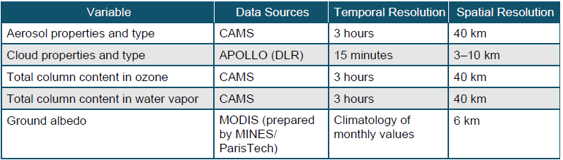
Perez/Clean Power Research

The Perez et al. (2002) method (herein referred to as the Perez State University of New York [Perez SUNY] model) evaluates GHI and DNI based on the concept that the atmospheric transmittance is directly proportional to the top-of-atmosphere planetary albedo (Schmetz 1989). This method is being applied to the GOES satellites and is currently available as the SolarAnywhere product from Clean Power Research.23 The concept of using satellite-based measurements of radiance assumes that the visible imagery demonstrates cloud cover for high levels of brightness and lower levels for clearer conditions (e.g., dark ground cover). Readers are referred to Perez et al. (2002) for additional details.

Vaisala Solar Data Set

3Tier (now Vaisala) developed a global solar radiation data set for both GHI and DNI. It follows the method of Perez et al. (2002) using independently developed algorithms. The revised Vaisala algorithms currently use the REST2 clear-sky model and other refinements. This data set is available for global locations at a 3-km resolution from 1997.24

Solargis

An advanced semi-empirical satellite model for the calculation of global and direct irradiances has been developed by Solargis (Cebecauer and Suri 2010) and implemented for the region covered by the Meteosat, GOES, and Himawari satellites covering land between latitudes 60° N and 50° S. The model philosophy is based on the principles of the Heliosat-2 calculation scheme (Hammer et al. 2003) and the model by Perez et al. (2002), and it is implemented to operationally process satellite data at a full spatial and temporal resolution. Compared to these earlier developments, the Solargis model includes various enhancements, such as a downscaling capability to take terrain effects and local variability into account.

EnMetSol Model

The EnMetSol method25 is a technique for determining the global radiation at ground level by using data from a geostationary satellite (Beyer, Costanzo, and Heinemann 1996; Hammer et al. 2003). It is used in combination with a clear-sky model to evaluate the three usual irradiance components. The key parameter of the method is the cloud index, n, which is estimated from the satellite measurements and related to the transmissivity of the atmosphere. The method is used for MFG, MSG, and GOES data. The EnMetSol method uses the SOLIS model (Müller et al. 2004) in combination with monthly averages of AOD (Kinne et al. 2005) and water vapor (Kalnay et al. 1996) as input parameters to calculate DNI or spectrally resolved solar irradiance. The DNI and DHI for all-sky conditions are derived from GHI with a beam-fraction model (Hammer et al. 2009; Lorenz 2007).

The method uses the clear-sky model of Dumortier (1998; see also Fontoynont et al. 1998) with Remund’s (2009) Meteonorm high-resolution database for the turbidity input. This model is also used to obtain near-real-time and forecasts of global tilted irradiance (GTI) as inputs for photovoltaic power prediction.

KNMI Cloud Physical Properties-Surface Insolation under Clear and Cloudy Skies and Solar Radiation Data Sets

KNMI operates a specific service, MSG-Cloud Physical Properties (CPP), by which near-real-time and historic satellite observations of cloud properties, surface radiation, and precipitation are provided to users. The data are retrieved from the Spinning Enhanced Visible and InfraRed Imager (SEVIRI) instrument onboard the EUMETSAT MSG satellite, and they are particularly attractive because of their high temporal frequency of 15 minutes combined with a 3-km by 3-km subsatellite spatial resolution. Retrieval algorithms have been developed in EUMETSAT’s Satellite Application Facility on Climate Monitoring (CM SAF) as well as other European and national projects. The basic retrieved parameters are cloud mask, cloud-top height, cloud thermodynamic phase, COD, particle effective radius, and water path.

The MSG-SEVIRI Surface Insolation under Clear and Cloudy Skies (SICCS) algorithm derives surface solar radiation (direct, diffuse, and global irradiance) using cloud physical properties. The SICCS products are available since 2004 at a 15-minute time interval. The CPP-SICCS products are provided at the SEVIRI pixels for the MSG full disk. The images and data can be obtained from the MSG-CPP website in near real time (http://msgcpp.knmi.nl/).

Validation results of hourly mean SEVIRI CPP-SICCS retrievals with observations at eight European BSRN stations yield median biases of 7 W/m2 (2%), 6 W/m2 (5%), and 1 W/m2 (1%) for global, direct, and diffuse irradiance, respectively; and median root mean square errors of 65 W/m2 (18%), 69 W/m2 (39%), and 52 W/m2 (34%) for global, direct, and diffuse irradiance, respectively. More detailed validation results are presented by Greuell et al. (2013).

Satellite Application Facility on Climate Monitoring Surface Radiation Products

The EUMETSAT’s CM SAF service and data portal provides various satellite-derived data records of cloud properties and surface solar radiation. The surface radiation products are part of the Cloud, Albedo, and surface RAdiation data set (CLARA) and the SARAH (Surface Radiation Data Set – Heliosat) data records. The global CLARA data record is based on polar-orbiting satellites, whereas the SARAH data record is based on geostationary Meteosat satellites. The CM SAF surface radiation data records are well documented and freely available as gridded netcdf data files; further information is available here:
https://www.cmsaf.eu/EN/Overview/OurProducts/Surface_Radiation_Albedo/Surface_Radiation _Products_node.html.

The CM SAF Surface Solar Radiation Data Set – Heliosat Edition 2.1 (SARAH-2.1) includes 30-minute, daily, and monthly mean data for solar surface irradiance (SIS); two surface direct irradiance parameters (SID) (direct horizontal radiation and DNI); sunshine duration (SDU) (daily, monthly sum); the spectrally resolved global irradiance (SRI) (monthly mean); and the effective cloud albedo (CAL) from 1983–2017 (Pfeifroth et al. 2018). Data are provided with a spatial resolution of 0.05° for the full disc of the Meteosat satellites at 0°, i.e., they cover Africa, Europe, and parts of South America. An adjusted Heliosat approach and the SPECMAGIC clear-sky model are used to estimate the irradiance from the geostationary satellite measurements
(Müller et al. 2012; 2015).

For the SARAH-2.1 data, the achieved accuracies of the monthly means as determined by comparison with reference measurements from the BSRN for the SIS, SID, and DNI parameters are 5.2 W/m2, 7.7 W/m2, and 16.4 W/m2, respectively. The daily accuracies are 11.7 W/m² for GHI, 17.1 W/m2 for SID, and 33.1 W/m2 for DNI. All values are based on the mean absolute difference between the SARAH-2.1 and the BSRN reference data.

To temporally extend the SARAH-2.1 climate data records, the CM SAF service provides consistent surface radiation data (SIS, SID, DNI, SDU) from 2018 onward with a delay of 5 days as part of the Interim Climate Data Record SARAH ICDR.

For the SARAH-E climate data record, satellite measurements from the Meteosat satellites located at the Indian Ocean Data Coverage have been used to estimate 60-minute, daily, and monthly surface irradiance (global and direct) from 1999–2016 (Amillo et al., 2014). The data cover most parts of Asia, Africa, and the western part of Australia and are provided with a spatial resolution of 0.05°.

The CLARA-A2 climate data record provides global data of cloud coverage and various cloud properties, surface radiation, and surface albedo from 1982–2015 (soon to be extended to mid-2019) (Karlsson et al. 2017a, 2017b). The SIS data are derived from the AVHRR measurements using a lookup-table approach (Müller et al. 2009) and are provided as daily and monthly means with a spatial resolution of 0.25°. The accuracy of the monthly and daily surface irradiance has been determined to be 9 W/m2 and 18 W/m2, respectively, by comparison with surface reference measurements from the BSRN.

EUMETSAT’s Satellite Application Facility on Climate Monitoring Cloud Property Data Sets

The CM SAF cloud products also include two records: one derived from the polar satellite instrument AVHRR and one from Meteosat. Details on the products, retrieval algorithms, and quality can be found in the Product User Manuals, the Algorithm Theoretical Basis Documents, and the Validation Reports
(https://www.cmsaf.eu/EN/Overview/OurProducts/CloudProducts/Cloud_Products_node.html). The products can be ordered via the web user interface.

Reuniwatt SICLONE Cloud Property Data Set

Reuniwatt offers SICLONE (Système d’Information pour l’analyse et la prévision des Configurations spatio-temporelLes des Occurrences NuageusEs), a cloud property data set containing cloud retrieval properties calculated with the Nowcasting Satellite Application Facility (NWCSAF) software (http://reuniwatt.com/en/applications/atmospheric-sciences/).

A comparison of cloud product databases was presented in 2019 at the European Meteorological Society conference: https://hal-mines-paristech.archives-ouvertes.fr/hal-02418087. In that study, the Heliosat-4 method was applied to three different cloud properties databases for the estimation of the surface downwelling shortwave irradiance. The first is the AVHRR Processing scheme Over cLouds, Land, and Ocean (APOLLO) database from the German Aerospace Center (DLR), which is implemented in the framework of the CAMS Radiation service. The second is the MSG-CPP product issued by the Royal Netherlands Meteorological Institute. The third is the CLAAS-2 data set generated by the German DWD in the framework of CM SAF.

Meteotest’s Meteonorm Satellite Irradiation Product
A model for the calculation of global irradiances was implemented for the region covered by the GOES-E, Meteosat, INDOEX, and Himawari satellites covering land between latitudes 65° N and 65° S. The model is based on the Heliomont method (Stöckli et al. 2013), which is itself based on the Heliosat approach. It is implemented to operationally process satellite data at a full spatial and temporal resolution. Data are adapted to ground sites with spatially interpolated linear regression functions. The model was further improved by Meteotest (Müller and Remund, 2018, Schmutz et al. 2020).