Introduction

Laboratory testing of soils and rocks is a fundamental element of geotechnical engineering. The complexity of testing required for a particular project may range from a simple moisture content determination to sophisticated triaxial strength testing. A laboratory test program should be well-planned to optimize the test data for design and construction. The geotechnical specialist, therefore, should recognize the projects issues ahead of time so as to optimize the testing program, particularly strength and consolidation testing.

Laboratory testing of samples recovered during subsurface investigations is the most common technique to obtain values of the engineering properties necessary for design. A laboratory-testing program consists of “index tests” to obtain general information on categorizing materials, and “performance tests” to measure specific properties that characterize soil behavior for design and constructability assessments (e.g., shear strength, compressibility, hydraulic conductivity, etc.). This course provides information on common laboratory test methods for soils and rocks including testing equipment, general procedures related to each test, and parameters measured by the tests.

1.1 Quality Assurance for Laboratory Testing

Laboratory testing will be required for most projects. Therefore, it is necessary to select the appropriate types and quantities of laboratory tests to be performed. A careful review of all data obtained during the field investigation and a thorough understanding of the preliminary design of geotechnical, structural and hydraulic features of the project are essential to develop an appropriately scoped laboratory testing program. In some cases owners may hire external testing laboratories to perform select tests. It is necessary that testing requests be clear and sufficiently detailed. Unless specialized testing is required, the owner should require that all testing be performed in accordance with the appropriate specifications for laboratory testing such as those codified in AASHTO and/or ASTM. Several tables are presented in this course that summarize various common tests for soils and rocks per AASHTO and ASTM standards. In order to assure that the results of laboratory testing are representative, several precautions must be taken before the tests themselves are performed. These precautions include: sample tracking, sample storage, sample handling to prevent sample disturbance, and sample selection. Discussion of each of these precautions follows.

1.1.1 Sample Tracking

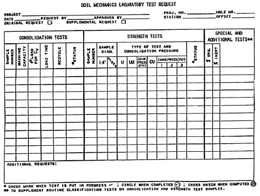
Whether the laboratory testing is performed in-house or is subcontracted, samples will likely be assigned a laboratory identification number that differs from the identification number assigned in the field. A list should be prepared to match the laboratory identification number with the field identification number. This list can also be used to provide tracking information to ensure that each sample arrived at the lab. When laboratory testing is requested, both the field identification number and the laboratory identification number should be used on the request form. An example request form is shown in Figure 1-1. A spreadsheet or database program is useful to manage sample identification data.

1.1.2 Sample Storage

Undisturbed soil samples should be transported and stored so that that the moisture content is maintained as close as possible to the natural conditions (AASHTO T 207, ASTM D 4220 and D 5079). Samples should not be placed, even temporarily, in direct sunlight. Shelby tubes should be stored in an upright position with the top side of the sample up in a humid room with relative humidity above 90%.

Long-term storage of soil samples in Shelby tubes is not recommended. As storage time increases, moisture will migrate within the tube. Potential for disturbance and moisture migration within the sample will increase with time, and samples tested 30 days after their retrieval should be noted on the laboratory data sheet. Excessive storage time can lead to additional sample disturbance that will affect strength and compressibility properties. Additionally, stress relaxation, temperature changes, and storage in a room with humidity below 90 percent may have detrimental effects on the samples. Long-term storage of soil samples should be in temperature- and humidity-controlled environments. The temperature control requirements may vary from sub freezing to ambient and above, depending on the environment of the parent formation. The relative humidity for soil storage normally should be maintained at 90 percent or higher to prevent moisture evaporation from the samples.

Long-term storage of soil samples in Shelby tubes is not recommended for another reason. During long term storage the sample tubes may corrode. Corrosion accompanied by adhesion of the soil to the tube may result in the development of such a large sidewall resistance that some soils may experience internal failures during extrusion. Often these failures cannot be seen by the naked eye; x-ray radiography (ASTM D 4452) will likely be necessary to confirm the presence of such conditions. If these samples are tested as “undisturbed” specimens, the results may be misleading.

1.1.3 Sample Handling

Careless handling of nominally undisturbed soil samples after they have been retrieved may cause major disturbances that could influence test results and lead to serious design and construction consequences. Samples should always be handled by experienced personnel in a manner that ensures that the sample maintains structural integrity and its natural moisture condition. Saws and knives used to prepare soil specimens should be clean and sharp. Preparation time should be kept to a minimum, especially where the maintenance of the moisture content is critical. Specimens should not be exposed to direct sun, freezing, or precipitation.

1.1.4 Effects of Sample Disturbance

As a soil sample is removed from the ground during a conventional soil investigation, its in-situ effective stress condition is being changed. In addition, nominally undisturbed specimens taken from samples obtained from drilled boreholes will become disturbed as a result of the drilling itself, sampling, sample extrusion, and sample trimming to form a specimen for testing. These processes will also change the effective stress condition in the soil sample, i.e., the effective stress in the soil at the time after a sample is trimmed and prepared for testing is different from that of the same soil in the ground. Therefore the utmost care should be taken to minimize the effect of these processes in order for the results of laboratory tests to represent the in-situ soil behavior accurately.

1.1.5 Specimen Selection

The selection of representative specimens for testing is one of the most important aspects of sampling and testing procedures. Selected specimens must be representative of the formation or deposit being investigated. The geotechnical specialist should study the boring logs, understand the geology of the site, and visually examine the samples before selecting the test specimens. Samples should be selected on the basis of their color, physical appearance, structural features and an understanding of the disturbance of the samples. Specimens should be selected to represent all types of materials present at the site, not just the worst or the best.

Samples with discontinuities and intrusions may fail prematurely in the laboratory. The first inclination would be to test these samples. However, if these features are small and randomly located, they may not necessarily cause such failures in the field. Therefore samples having such local features should be noted, but not necessarily selected for testing since such samples may not be representative of the stratum in terms of its response to applied loads.

Certain considerations regarding laboratory testing, such as when, how much, and what type, can be decided only by an experienced geotechnical specialist. The following minimal criteria should be considered when the scope of the laboratory testing program is being determined:

• Project type (bridge, embankment, building, reconstruction or new construction, etc.)
• Size of the project (geographic extent).
• Loads to be imposed on the foundation soils (geometry, type, direction and magnitude).
• Performance requirements for the project (e.g., settlement and lateral deformation limitations).
• Vertical and horizontal variations in the subsurface profile as determined from boring logs and visual identification of subsurface material types in the laboratory.
• Known or suspected peculiarities of subsurface strata at the project location (e.g.,swelling soils, collapsible soils, organics, etc.)
• Presence of visually observed intrusions, slickensides, fissures, concretions, etc.

The selection of tests should be considered preliminary until the geotechnical specialist is satisfied that the test results are sufficient to develop reliable subsurface profiles and provide the parameters needed for design.

1.2 Laboratory Testing for Soils

Table 1-1 provides a listing of commonly-performed soil laboratory tests. Tables 1-2 and 1-3 provide a summary of typical soil index and performance tests, respectively. Additional information on these tests is provided in subsequent sections.

1.3 Laboratory Index Tests for Soils

1.3.1 General

Data generated from laboratory index tests provide an inexpensive way to assess soil consistency and variability among samples collected from a site. Information obtained from index tests is used to select samples for engineering property testing as well as to provide an indicator of general engineering behavior. For example, a soil with a high plasticity index (PI) can be expected to have high compressibility, low hydraulic conductivity, and high swell potential. Common index tests discussed in this course include moisture content, unit weight (wet density), Atterberg limits, particle size distribution, visual classification, specific gravity, and organic content. Index testing should be conducted on each type of soil material on every project. Information from index tests should be assessed prior to a final decision regarding the specimens selected for subsequent performance testing.

1.3.2 Moisture Content

The moisture (or water) content test is one of the simplest and least expensive laboratory tests to perform. Moisture content is defined as the ratio of the weight of the water in a soil specimen to the dry weight of the specimen. Natural moisture contents (w_n) of sands are typically 0 ≤ w_n ≤ 20 %, whereas for inorganic and insensitive silts and clays, the typical range is 10 ≤ w_n ≤ 40 %. However, for clays it is possible to have more water than solids (i.e., w_n > 100%), depending upon the mineralogy, formation environment, and structure of the clay. Therefore, soft and highly compressible clays, as well as sensitive, quick, or organically rich clays, can exhibit water contents in the range of 40 ≤ w_n ≤ 300 % or more.

Moisture content can be tested a number of different ways including: (1) a drying oven (ASTM D 2216); (2) a microwave oven (ASTM D 4643); or (3) a field stove or blowtorch (ASTM D 4959). While the microwave or field stove (or blowtorch) methods provide a rapid evaluation of moisture content, potential errors inherent with these methods require confirmation of results obtained by using ASTM D 2216. The radiation heating induced by the microwave oven and the excessive temperature induced by the field stove may release water entrapped in the soil structure (adsorbed water) that would normally not be released at 230o F (110o C), the maximum temperature specified by ASTM D 2216. Therefore, the microwave oven and field stove methods may yield greater values of moisture content than would occur from ASTM D 2216. Field measurements of moisture content often rely on a field stove or microwave due to the speed of testing. For control of compacted material, it is common to use a nuclear gauge (ASTM D 3017) in the field to assess moisture contents rapidly. Nuclear gage readings may indicate widely varying moisture contents for micaceous soils, i.e., soils containing a significant amount of mica particles. Results from nuclear techniques should be “calibrated” or confirmed by using the drying oven method (ASTM D 2216).

Moisture contents of soils as determined from in-situ moisture content tests may be altered during sampling, sample handling, and sample storage. Because the top end of the sample tube may contain water or collapse material from the borehole, moisture content tests should not be performed on material near the top of the tube. Also, as storage time increases, moisture will migrate within a specimen and lead to altered values of moisture content. If the sample is not properly sealed, moisture loss through drying of the sample will likely occur.

1.3.3 Unit Weight

The terms density (ρ) and unit weight (γ) are often incorrectly used interchangeably. The correct usage is that density implies mass while unit weight implies weight measurements. Density and unit weight are related through the gravitational constant (g) as follows: γ = ρg. In this document they will be referenced as “density (unit weight)” if the usage is independent of the specific definition.

In the laboratory, soil unit weight and mass density are easily measured on tube (undisturbed) samples of natural soils. The moist (total) mass density is ρ_t = M_t/V_t, where M_t is the total mass of the soil sample including the mass of the moisture in the pores and V_t is the total volume of the soil sample. Similarly the dry mass density is given by ρ_d = M_s/V_t , where Ms is the mass of the solid component of the soil sample and V_t is the total volume of the soil sample. Likewise, the moist unit weight is γ_t = W_t/V_t, where W_t is the total weight including the weight of the water in the pores and V_t is the total volume of the soil sample. Similarly, the dry unit weight is defined as γ_d = W_s/V_t where W_s is the weight of the solid component of the soil sample and V_t is the total volume of the soil sample. The relationship between the total and dry mass density and unit weight in terms of natural moisture content, w, is given by:

Since γ = ρg the relationship between total and dry unit weight is given by:

Field measurements of soil mass density (unit weight) are generally restricted to shallow surface samples such as those obtained during placement of compacted fills. In those cases, field measurements of soil mass density (unit weight) can be accomplished by using drive tubes (ASTM D 2937), the sand cone method (ASTM D 1556), or a nuclear gauge (ASTM D 2922). To obtain unit weights or mass densities with depth, either high-quality thin-walled tube samples must be obtained (ASTM D 1587), or relatively expensive geophysical logging by gamma ray techniques (ASTM D 5195) can be employed.
Table 5-4 presents typical unit weights along with a range of void ratios for a variety of soils.

1.3.4 Particle Size Distribution

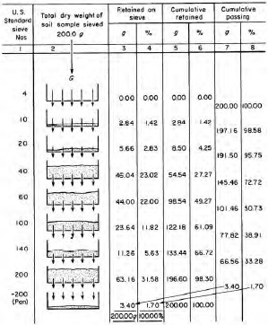
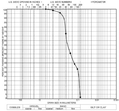
Particle size distributions by mechanical sieve and hydrometer analyses are useful for soil classification purposes. Procedures for grain size analyses are contained in ASTM D 422 and AASHTO T88. Testing is accomplished by shaking air-dried material through a stack of sieves having decreasing opening sizes. Each successive screen in the stack has a smaller opening to capture progressively smaller particles. The amount retained on each sieve is collected, dried and weighed to determine the percentage of material passing that sieve size. An example of how to determine the grain size distribution from sieve data is shown in Figure 1-2. The grain size distribution curve corresponding to the data in Figure 1-2 is presented in Figure 1-3.

Testing of the finer grained particles is accomplished by suspending the chemically dispersed particles in a water column and measuring the change in the specific gravity of the liquid as the particles fall from suspension. This part of the test is commonly referred to as a hydrometer analysis.

Obviously, obtaining a representative specimen is an important aspect of this test. When soil samples are dried or washed for testing, it may be necessary to break up the soil clods. Care should be taken to avoid crushing of soft carbonate or sand particles. If the soil contains a substantial amount of fibrous organic materials, these may tend to plug the sieve openings during washing. The material settling over the sieve during washing should be constantly stirred to avoid plugging.

Particle size testing is relatively straightforward, but the results can be misleading if procedures are not performed correctly and/or if equipment is not maintained in good working condition. If the sieve screen is distorted, large particles may be able to pass through sieve openings that typically would retain the particles. Material lodged within the sieve from previous tests could become dislodged during shaking, thereby increasing the weight of material retained on the following sieve. Therefore, sieves should be cleaned thoroughly after each test. A wire brush may distort finer sieve meshes during cleaning, so a plastic brush should be used to clean the U.S. No. 40 (0.425 mm) sieve and finer. Openings of fine mesh No. 200 sieve (0.075 mm)) are easily distorted as a result of normal handling and use. Therefore, fine-mesh sieves should be replaced often. A simple way to determine whether sieves should be replaced is to examine the stretch of the sieve fabric on its frame periodically. The fabric should remain taut; if it sags, it has been distorted and should be replaced. A common cause of serious errors is the use of “dirty” sieves. Some soil particles, because of their shape, size or adhesion characteristics, have a tendency to lodge in the sieve openings. This is especially true of the fine mesh sieves.

Representative samples of fine-grained soils (i.e., samples containing more than 50% of particles with diameter less than the U.S. No. 200 sieve size (075 mm ) should not be oven dried prior to testing because some particles may cement together leading to a calculated lower fines content from mechanical sieve analyses than is actually present. When fine-grained particles are a concern, the wash sieve method (ASTM D 1140) should be performed to assess the fines content.

If the clay-size content is an important parameter, hydrometer analyses should be performed even though the hydrometer test provides only approximate results due to oversimplified assumptions. However, the results can still be used as a general index of silt and clay-size content. Depending upon the chemical makeup of the fine grained particles, the traditional sodium hexametaphosphate solution used to disperse the clay-size particles may not provide adequate dispersion. If the clay-size particles are not dispersed, the hydrometer data leads to the interpretation of a lower than actual clay-size content. In some cases the concentration of the dispersing agent may need to be increased or a different dispersing agent may need to be used. If the sieve and hydrometer analyses are performed correctly, the gradation curve should be continuous over a range that includes all particle sizes.

1.3.4.1 Sand Equivalent

The sand equivalent test is a rapid test to show the relative proportions of fine dust or claylike materials in aggregate (or soils). A sample of aggregate passing the No. 4 sieve (4.75-mm) sieve and a small amount of flocculating solution are poured into a graduated cylinder and are agitated to loosen the claylike coatings from the sand particles. The sample is then irrigated with additional flocculation solution forcing the claylike material into suspension above the sand. After a prescribed sedimentation period, the height of flocculated clay and height of sand are determined. The sand equivalent is determined from the ratio of the height of the sand to height of the clay and expressed as a percentage. Cleaner aggregates will have higher sand equivalent values. For asphalt pavements, agencies often specify a minimum sand equivalent around 25 to 35 (Roberts, et al., 1996). Higher values are used in case of compacted structural fill which may support structures.

1.3.5 Atterberg Limits

The Atterberg limits of a fine grained soil represent the moisture content at which the physical state of the soil changes. The tests for the Atterberg limits are referred to as index tests because they serve as an indication of several physical properties of the soil, including strength, permeability, compressibility, and shrink/swell potential. These limits also provide a relative indication of the plasticity of the soil, where plasticity refers to the ability of a silt or clay to retain water without changing state from a semi-solid to a viscous liquid. In geotechnical engineering practice, the Atterberg limits generally refer to the liquid limit (LL), plastic limit (PL), and shrinkage limit (SL). In this course the definition is extended further in terms of quantifiable parameters that permit their measurements in the laboratory. These quantifiable definitions are as follows:

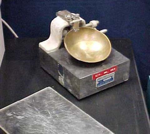
• Liquid Limit (LL) – This limit represents the moisture content at which any increase in moisture content will cause a plastic soil to behave as a viscous liquid. The LL is defined as the moisture content at which a standard groove cut in a remolded sample will close over a distance of ½-inch (13 mm) at 25 blows of the liquid limit device (Figure 1-4). The test is performed on material passing a US Standard No. 40 sieve(0.425 mm). During the test the material is brought to various moisture contents, usually by adding water. The plot of moisture contents vs. blows required to close the groove is called a “flow curve” and the value of the liquid limit moisture content is obtained from the flow curve at 25 blows.

• Plastic Limit (PL) – This limit represents the moisture content at which the transition between the plastic and semisolid state of a soil occurs. The PL is defined as the moisture content at which a thread of soil just crumbles when it is carefully rolled out by hand to a diameter of 1/8-inch (3 mm).
• Shrinkage Limit (SL) – This limit represents the moisture content corresponding to the change between the semisolid to solid state of the soil. The SL is also defined asthe moisture content at which any further reduction in moisture content will not result in a decrease in the volume of the soil.

Based on the above index values, there are two useful related indices, namely, the Plasticity Index (PI) and the Liquidity Index (LI), as follows:

where w is the natural (in-situ) water content of the soil. Numerous engineering correlations have been developed that relate PI and LI to clay soil properties, including undrained and drained strength to PI and compression index to LI.

Another useful index proposed by Skempton (1953) based on the proportion of clay and PI is known as the “Activity Index.” The activity index of a clay soil is denoted by A and is generally defined as follows:

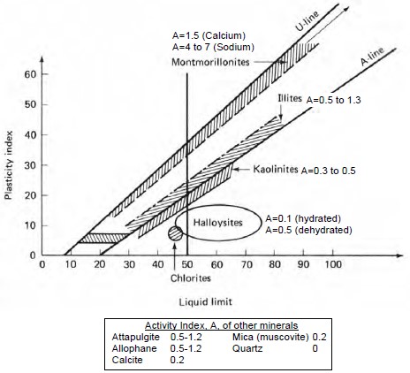
where CF is the clay fraction is usually taken as the percentage by weight of the soil with a particle size less than 0.002 mm. Clays with 0.75 < A < 1.25 are classified as “normal” clays while those with A < 0.75 are “inactive” and A > 1.25 are “active.” Values of activity index, A, can be correlated to the type of clay mineral that, in turn, provides important information relative to the expected behavior of a clay soil. A clay soil that consists predominantly of the clay mineral montmorillonite behaves very differently from a clay soil composed predominantly of kaolinite. Figure 1-5 also shows the activities of various clay minerals and their location on the Casagrande’s plasticity chart. The symbol for the activity index (A) in Figure 1-5 should not be confused with the “A-line” also shown in the figure.

Modified Activity Index, A_m: Based on their studies regarding the swell potential of compacted natural and artificial clay soils, Seed et al. (1962) proposed that for natural clay soils compacted as per the requirements of ASTM D 698 and Atterberg limits determined by ASTM D 4318 (AASHTO T 89, T 90), a Modified Activity Index, A_m, defined as follows is more appropriate:

The above definition is used to define the swell potential of soils (see Section 1.7).

1.3.5.1 Significance of the “A-line” and “U-line” on Plasticity Chart

The equation for the A-line and U-line are:

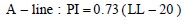
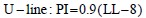
The A-line generally separates soils whose behavior is more claylike (points plotting above the A-Line) from those that exhibit a behavior more characteristic of silt (points plotting below the A-line). The A-line also separates organic (below) from inorganic (above) soils. The LL = 50 line generally represents the dividing line between silt, clay and organic fractions of the soil that exhibit low plasticity (LL<50) and high plasticity (LL>50). The U-line shown in Figure 5-5 represents the upper range of PI and LL coordinates that have been found for soils. When the limits of any soil plot above the U-line, the results should be considered spurious and the tests should be rerun. Note that in Figure 5-5 the clay mineral montmorillonite plots well above the A-line and just below the U-line. If a soil plots in this range, it probably contains a significant amount of the clay mineral montmorillonite that expands in presence of water.

1.3.6 Specific Gravity

The specific gravity of solids (G_s) is a measure of solid particle density and is referenced to an equivalent volume of water. Specific gravity of solids is defined as G_s = (M_s/V_s)/ ρ_d where M_s is the mass of the soil solids and V_s is the volume of the soil solids and ρ_d is the mass density of water = 1,000 kg/m³ or 1 Mg/m³. This formulation represents the theoretically correct definition of specific gravity and can be rewritten as G_s = ρ_s / ρ_d.

However, since γ = ρg the gravitational constant appears in both the numerator and denominator of the expression and the equation for G_s can also be given as G_s = γ_s/γ_w where γ_s = unit weight of solid particles in the soil mass and γ_w = unit weight of water = 62.4 pcf (1,000 kg/m³ or 1 Mg/m³).

The typical values of specific gravity of most soils lie within the narrow range of G_s = 2.7 ± 0.1. Exceptions include soils with appreciable organics (e.g., peat), ores (e.g., mine tailings), or calcareous (high calcium carbonate content) constituents (e.g., caliche). It is common to assume a reasonable G_s value within the range listed above for preliminary calculations. Laboratory testing by AASHTO T100 or ASTM D 854 or D 5550 can be used to confirm the magnitude of G_s, particularly on projects where little previous experience exists and unusually low or high unit weights are measured.

1.3.7 Organic Content

A visual assessment of organic materials may be very misleading in terms of engineering analysis. Laboratory test method AASHTO T194 or ASTM D 2974 should be used to evaluate the percentage of organic material in a specimen where the presence of organic material is suspected based on field information or from previous experience at a site. The test involves weighing and heating a previously dried sample to a temperature of 824°F (440°C) and holding this temperature until no further change in weight occurs. At this temperature, the organics in the sample turn to ash and the sample is re-weighed. Therefore, with the assumption that the weight of the ash is negligible, the percentage of organic matter is the ratio of the difference in weight before and after heating the sample to 824°F (440°C) to the weight of the original dried sample. The sample used for the test can be a previously dried sample from a moisture content evaluation. Usually organic soils can be distinguished from inorganic soils by their characteristic odor and their dark gray to black color. In doubtful cases, the liquid limit should be determined for an oven-dried sample (i.e., dry preparation method) and for a sample that is not pre-dried before testing (i.e., wet preparation method). If drying decreases the value of the liquid limit by about 30 percent or more, the soil may usually be classified as organic (Terzaghi, et al., 1996).

Soils with relatively high organic contents have the ability to retain water. Water retention may result in higher moisture content, higher primary and secondary compressibility, and potentially higher corrosion potential. Organic soils may or may not be relatively weak depending on the nature of the organic material. Highly organic fibrous peats can exhibit high strengths despite having a very high compressibility. In some instances such soils may even exhibit tensile strength.

1.3.8 Electro Chemical Classification Tests

Electro chemical classification tests provide the geotechnical specialist with quantitative information related to the aggressiveness of the soil conditions with respect to corrosion and the potential for deterioration of typical foundation materials. Electro chemical tests include determination of pH, resistivity, sulfate ion content, sulfides, and chloride ion content. Depending on the application, limits of these electro chemical properties are established based on various factors such as corrosion rates for metals and disintegration rates for concrete. Tests to characterize the aggressiveness of a soil environment are important for design applications that include metallic elements, especially for ground anchors comprised of high strength steel and for metallic reinforcements in mechanically stabilized earth walls. ASTM and AASHTO test procedures are listed under “Corrosivity (Electrochemical)” in Table 1-1.

1.3.9 Laboratory Classification

In addition to field identification (ASTM D 2488), soils should be classified in the laboratory by using the Unified Soil Classification System (USCS) in accordance with ASTM D 2487 or by the AASHTO soil classification system in accordance with AASHTO T 145. The USCS will be used throughout the remainder of this document. Classification in the laboratory occurs in a controlled environment and more time can be spent on this classification than the identification exercise performed in the field. Laboratory and/or field identification is also important so that defects and features of the soil can be recorded that would not typically be noticed from index testing or standard classification. Some of the features include degree of calcium carbonate cementation, mica content, joints, and fractures.

1.4 Consolidation Testing

1.4.1 Process of Consolidation

Consolidation is a time-dependent decrease in the volume of a soil mass under applied loading. In highway design, static loading is represented by the permanent load placed on the soil by embankments and structures. Depending on the configuration of the load and the subsurface conditions, the stress increase due to the externally applied loads may extend below the water table where all the voids are filled with water. An applied load will cause the soil grains to readjust to a more compact position to carry the load. This readjustment cannot take place until the water, which is incompressible, escapes from the voids.

The rate of the readjustment of the soil particles is a function of the void size, which controls the rate at which the water can escape from the voids. The settlement associated with the readjustment of the soil particles due to migration of water out of the voids is known as primary consolidation.

The amount of primary consolidation will depend on the initial void ratio of the soil. The greater the initial void ratio, the more water that can be squeezed out, and the greater the primary consolidation. The rate at which primary consolidation occurs is dependent on the rate at which the water is squeezed out of the soil voids. Secondary compression occurs after primary consolidation is complete. Secondary compression occurs under constant load. It is caused by the soil particles reorienting or deforming under constant load at a very slow rate. This process is known as “creep” and it occurs in most soils when they are subjected to long-term applied loads. Therefore, secondary compression is also a time-dependent process. However, secondary compression is not dependent on water being squeezed out of the soil as is consolidation. That is why it is called “secondary compression” and not “secondary consolidation.” Primary consolidation accounts for the major portion of settlement in saturated fine-grained soils. Primary consolidation and secondary compression both contribute significantly to settlements in organic soil.

Some natural deposits of fine-grained soils experienced compression in geologic history due to the weight of glaciers, due to the weight of overlying soil that has been eroded, or due to desiccation. Since their void ratios were substantially reduced in the past by these processes, these soils are less compressible today. Such soils are called “preconsolidated” or “overconsolidated” since they have been subjected to greater stresses in the past than exist at present. This concept is important because overconsolidated soils can be reloaded such as by the load from an embankment or bridge substructure without settling appreciably until the currently applied load exceeds the preconsolidation load. Saturated fine-grained soil deposits, which have never consolidated under loads other than the current loads, are called “normally consolidated.” On the other end of the spectrum, soils whose present loading induces stresses in the soil that are greater than the maximum effective stress they have experienced in the past are called “under consolidated.” This means that the consolidation process under the existing loading is on-going and the soil will continue to consolidate until that process is complete, even if no additional loads are applied.

1.4.2 Consolidation Testing

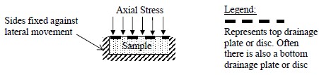
To predict the amount of consolidation in saturated fine-grained and organic soils, adequate testing must be performed. An undisturbed soil sample should be obtained in the field with a Shelby tube sampler. The oedometer or one-dimensional consolidometer is the primary laboratory equipment used to evaluate consolidation and settlement potential of fine-grained soils. A consolidation test is typically performed on a specimen obtained from an undisturbed sample retrieved from the deposit of fine-grained soils to evaluate the consolidation characteristics of the soil and define the settlement-time relationship of the in-situ soils under proposed foundation loads. The equipment for a consolidation test includes:

1. A loading device that applies a vertical load to the soil specimen,
2. A metal ring (fixed or free) that laterally confines the soil specimen and restricts deformation to the vertical direction only (i.e., only one-dimensional compression is modeled),
3. Porous discs placed on the top and bottom of the sample to allow the sample to drain,
4. A dial indicator or linear variable differential transducer (LVDT) to measure vertical displacement. Properly calibrated, each device should provide the same accuracy, but the electronic output of an LVDT can be incorporated into an automated recording system for quicker, more efficient, and higher resolution readings.
5. A timer to assess the duration of loading increments. Monitoring of time for manual systems can be accommodated by use of a wall clock with a second hand. The internal clock of a computer is used for automated systems
6. A surrounding container to permit the specimen to remain submerged during the test.

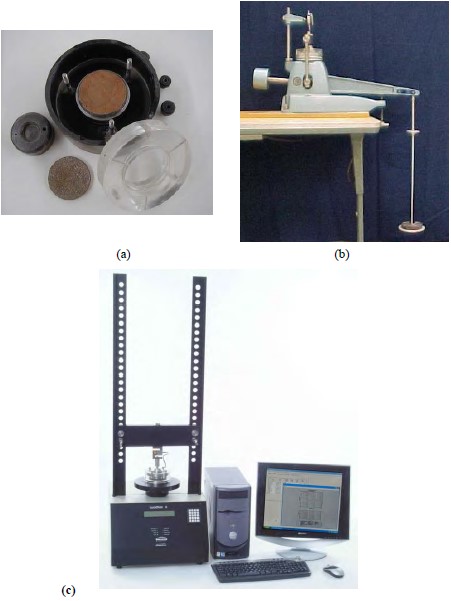
Figure 1-6 shows a schematic of a consolidation test. The consolidation-loading device may be a weighted lever arm as shown in Figure 1-7b, a pneumatic device, or an automated loading frame as shown in Figure 1-7c. Automated loading frames are recommended for use in production testing because they provide the most flexibility in testing options. The pneumatic device provides flexibility in loads and load increment ratios (LIR) that can be applied during testing. A weighted lever arm provides a robust, relatively simple system for consolidation testing, however, because data are generally recorded manually, it is difficult to expedite testing or vary the loading schedule since data reduction cannot typically be performed in real time.

Consolidation cells may be either fixed ring or floating ring. Friction and drag are created in the ring as the specimen compresses in relation to the ring. In a fixed ring test the sample compresses from the top only, potentially resulting in high incremental side shear forces. In a floating ring test the sample compresses from the top and bottom thus providing the advantage of minimizing drag forces. However, the floating ring method has the following disadvantages: it is more difficult to set up; it has the potential for sidewall leakage that would result in an inaccurate assessment of the rate of consolidation, and soil may squeeze out near the junction of the sidewall and the bottom porous disc. Because of these disadvantages, the fixed ring method is most commonly used.

1.4.3 Procedures

The consolidation properties of fine-grained soils are evaluated in the laboratory by using the one-dimensional consolidation test. The most common laboratory method is the incremental load (IL) method (ASTM D 2435). The weighted lever arm oedometer shown in Figure 1-7b is commonly used for performing the procedure. The automated load-frame apparatus shown in Figure 1-7c provides higher quality test results compared to the weighted lever apparatus. High-quality undisturbed samples obtained by using Shelby tubes (ASTM D 1587), piston samplers, or other special samplers are preferred for laboratory consolidation tests.

1.4.4 Presentation and Understanding the Consolidation Test Results

The consolidation test should be run in such a way that sufficient time is allowed for the applied pressure (total stress) increment to be transmitted from the pore water, where it acts initially as a excess pore water pressure, to the soil structure where it ultimately becomes an applied effective stress increment. The time it takes for this transfer to occur is the basis for the process being called “consolidation” and not “compression.” Therefore, the effective stress corresponding to the applied pressure is generally plotted versus void ratio. The resulting “consolidation curve” permits an evaluation of the preconsolidation pressure and values for other parameters pertaining to the consolidation characteristics of the soil sample.

Plots of void ratio versus effective pressure on arithmetic and logarithmic scales are shown in Figure 1-8. The semi log plot is more widely used in practice and will be used in subsequent sections of this manual. The consolidation curve on the void ratio versus semi log pressure plot is commonly referred to as the “e-log p” relationship. As shown on Figure 1-8, the slope of the loading portion of the e-lop p curve is called the compression index, which is denoted by the symbol C_c. The slope of the re-load portion of the e-log p curve is called the re-compression index; it is denoted by the symbol C_r.

Some geotechnical specialists prefer to use a plot of percent strain versus log of pressure instead of the e-log p plot. In this case the slope of the virgin compression portion of the consolidation curve is called the modified compression index denoted by the symbol Ccε and the slope of the rebound portion of the curve is called the modified recompression index denoted by the symbol C_rε. The modified indices reflect the relationship between strain and void ratio, i.e., strain (ε) = Δe/(1+e_o). Therefore, to convert the strain-based indices (C_cε and C_rε) to the void-ratio-based indices (C_c and C_r) multiply the strain based values by (1 + e_o). Void-ratio-based values (e-log p) will be used in the remainder of this manual.

Analysis of consolidation test data allows the engineer to determine:

1. Initial Void Ratio (e_o)The value of the initial void ratio is very important because it defines the amount of void space at the start of the loading. It is this initial void space that will be reduced as the water is squeezed out of the voids with time. The initial void ratio e_o is a key parameter used in settlement computations to determine the magnitude of settlement.

   

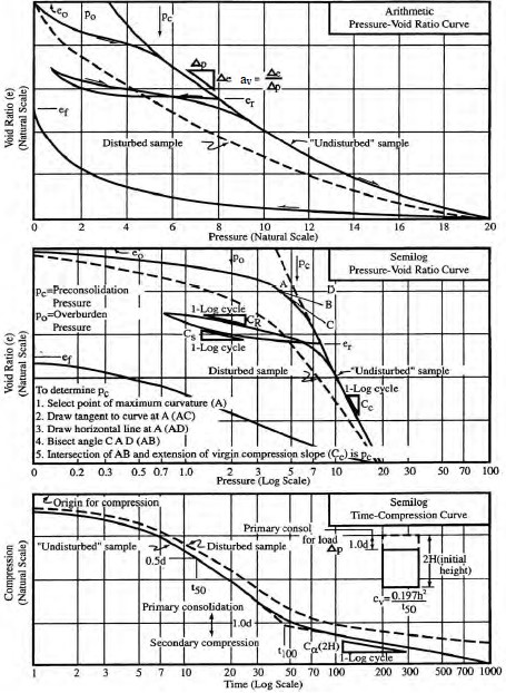
2. Preconsolidation Pressure (p_c)The e-log p relationship generally displays a distinct break at approximately the maximum past effective stress (p_c). The graphical technique developed by Casagrande (1936) is generally used to determine the value of p_c, which is known as preconsolidation pressure. The Casagrande procedure is included in the middle portion of Figure 1-8.The maximum effective stress to which a soil has been loaded in the past will have a major influence on the amount of settlement to be expected under a proposed loading. In fact, 10 times more settlement may occur in a normally consolidated soil than a preconsolidated soil for equal load increments up to the preconsolidation pressure. Values of preconsolidation pressure should be carefully established for the entire depth of the fine-grained soil deposit under consideration. Normally, a minimum, maximum and most probable value of p_c will be determined from laboratory test results and plotted as a range with depth.
3. Compression Index (C_c)The slope of the consolidation curve beyond pc is called the compression index (C_c). It is a measure of the load-deformation characteristic of the soil during “virgin” compression.
4. Recompression Index (Cr)An unload/reload segment of the consolidation curve is also shown in Figure 1-8. The slope of the reload curve is called the recompression index (C_r). It is a measure of the load-deformation characteristic of the soil upon reloading after some amount of load release. As is obvious in Figure 1-8, the slope of the reload portion of the consolidation curve is not as steep as the slope of the virgin portion of the curve since the void ratio change accompanying the virgin loading is unrecoverable. Figure 1-8 also shows that if, upon reloading, the applied pressure exceeds the pressure from which the soil was unloaded, the slope of the reload curve reverts back to the virgin compression slope, C_c. In general, C_c ≈ 10 C_r.
5. Coefficient of Consolidation (c_v)The coefficient of consolidation is an indicator of the rate of drainage during consolidation. The value may be determined by the t₅₀ (log time) method or the t₉₀ (square root of time) method. As shown in the bottom portion of Figure 1-8, the compression-log time curve for a given load increment is used to determine the coefficient of consolidation (c_v), which is a measure of the time rate of primary consolidation. The value of c_v is determined for each load increment. These values are sometimes plotted on a separate axis below the consolidation curve
6. Secondary Compression Index (C_α)Of great importance in organic materials, secondary compression may account for the majority of settlement that takes place over a long period of time in such soils. The compression-log time curve for a given load increment is used to determine the secondary compression index (C_α), which is basically the slope of the curve over one log cycle beyond the time required for primary consolidation (t₁₀₀) as shown in the bottom portion of Figure 1-8.
7. Effects of Sample Disturbance on Consolidation Test ResultsThe influence of sample disturbance on consolidation test results is shown on Figure 1-8 by the dashed lines. The dash lines indicate that disturbance:

1. Eliminates the distinct break in the e-log p curve at the preconsolidation pressure (p_c).
2. Lowers the estimated value of the preconsolidation pressure (p_c) and the measured value of the compression index (C_c).
3. Decreases the measured values of c_v.
4. Increases the recompression index (C_r).
5. Decreases the secondary compression index (C_α).

The general effects of disturbance are (a) under- or over-prediction of the magnitude of expected settlement and (b) over-prediction of the time for its occurrence.

The importance of the consolidation test results as applied to design is summarized below. The test results may be applied to project design after a series of tests have been completed to represent the total depth of the fine-grained soil deposit. The two most important predictions are:

1. The amount of settlement. The value is determined by analyzing the consolidation curve between the existing overburden pressure and the final pressure induced by the highway load at various depths. The amount of settlement may vary dramatically depending upon the maximum past pressure to which the soil has been loaded. The total amount of long-term settlement should include an estimate of settlement due to secondary compression, especially for times past the time for 100% primary consolidation if that is less than the design life of the constructed facility.
2. The time for settlement. The time for primary consolidation to occur may be estimated from the results of the compression versus time plots at loads between the overburden pressure and final pressure induced by the applied load. The important factors in the settlement-time relationship are:

1. Time required is proportional to the square of the longest distance required for water to drain from the deposit. This distance is the thickness of the layer if water drains in one direction only (generally vertically upward to the surface), and one-half the layer thickness if more permeable soils exist above and below the consolidating layer.
2. Time required for consolidation varies inversely with the coefficient of consolidation.
3. Rate of settlement decreases as time increases.

1.4.5 Comments on the Consolidation Tests

The consolidation test results are necessary to assess the consolidation properties of the soil. As will be shown in subsequent sections of this document, the consolidation test is one of the most important tests for fine-grained soil as it provides data regarding stress history and compressibility. It is important to consider all laboratory testing variables and their potential effects on the values of soil properties computed from the test results. Information that will need to be provided to a laboratory for a consolidation test includes the loading schedule (i.e., magnitude and duration of loads). It is important to evaluate the loading schedule to be used, especially the duration of loading since time is required for the applied total stress increment to be transferred from the pore water to the soil structure so that it becomes an effective stress acting on the soil mass. Important issues related to consolidation tests are discussed below.

• Loading Sequence: The loading sequence selected for a consolidation test will depend on the type of soil being tested and the particular application being considered for the project (e.g., embankment, shallow foundation). The selection of a loading sequence should never be left to the discretion of the laboratory. As an example, if the clay soil is heavily over consolidated, it is possible that a laboratory-determined maximum load for the consolidation test will not be sufficient to exceed pc.
• Range of Applied Loads: The range of applied loads for the test should well exceed the effective stresses that are required for settlement analyses. This range should cover the smallest and largest effective stresses anticipated in the field and will depend on depth, foundation loads, and excavations. The anticipated preconsolidation stress should be exceeded by at least a factor of four during the laboratory test. If the preconsolidation stress is not significantly exceeded during the loading schedule, pc, and C_c (or C_cε) may be underestimated due to specimen disturbance effects.
• Load Increment Ratio (LIR): By definition the LIR= Δσ/σ_initial where Δσ is the incremental stress and σ_initial is the previous stress. A LIR=1 corresponds to a doubling of the vertical stress applied to the specimen at each successive load increment during a consolidation test. A LIR of 1 is commonly used for most tests. Experience with soft sensitive soils suggests that as the stress approaches the value of p_c, a smaller LIR will facilitate a better estimate of p_c. Typically, laboratories provide a unit cost for a consolidation test that may be based on 6 to 8 load increments with a separate cost for each additional increment.
• Unload-Reload Cycle: It is recommended that an unload-reload cycle be performed, especially for cases where accurate settlement predictions are required, specifically to obtain a value for C_r. Since most samples will inevitably be somewhat disturbed, a C_r value based on the initial loading of a consolidation test sample will be greater than that for an undisturbed sample, resulting in an overestimation of settlements in the over consolidated region. A value of C_r based on an unload-reload cycle is more likely to be representative of the actual behavior of the soil in the over consolidated region.
• Duration of Load Increment: The duration of each load increment should be selected to ensure that the sample is approximately 100 percent consolidated prior to application of the next load increment. For relatively low to moderate plasticity silts and clays, durations of 3 to 12 hours will be appropriate for loads in the normally consolidated range. For fibrous organic materials, primary consolidation may be completed in 15 minutes for each load increment. For high plasticity materials, the duration for each load increment may need to be 24 hours or more to ensure complete primary consolidation and to evaluate secondary compression behavior. Conversely, primary consolidation may occur in less than 3 hours for loads less than p_c. If the time period is too short for a given load increment (i.e., the sample is not allowed to achieve approximately 100 percent consolidation before the next load increment is applied), then values of C_c may be underestimated and values of cv may be overestimated. The duration of time required, however, can be optimized by using pneumatic, hydraulic, or electro-mechanical loading systems that include automated loading and data acquisition systems. Continuous deformation versus time measurements and the square root of time method can be used to estimate the beginning and end of primary consolidation during the test. Once the end of primary consolidation is detected, the system can automatically apply the next load increment. Alternatively, some laboratories can provide real-time deformation versus log time plots to enable the engineer to evaluate whether 100 percent primary consolidation has been achieved.
• Secondary Compression: In cases where secondary compression is important (e.g., organic soils), secondary compression should be assessed on the basis of the deformation versus log-time response. The consolidation test for each load increment should be run long enough to establish a linear trend between vertical displacement and log time.

1.4.6 Useful Correlations between Consolidation Parameters and Index Values

This section presents some useful correlations between consolidation parameters and other index values. These correlations can be used by the designer to check the validity of the laboratory tests results or to develop a prediction of the range of values of consolidation parameters that can be expected from yet-to-be performed consolidation tests. It must be emphasized that predictions based on correlations should never be substituted for proper testing and that any assumptions regarding consolidation parameters should always be verified through testing.

1.4.6.1 Compression Index, C_c

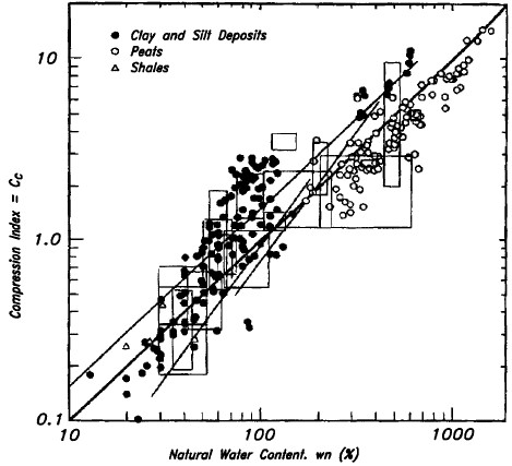
Over 70 different equations have been published for correlating C_c with the index properties of clays. Table 1-5 lists some of the more useful correlations. Figure 1-9 shows correlations between natural water content and C_c for fine-grained soils, peats and shales. Note that the coordinates in Figure 1-9 are both logarithmic so that values of C_c can vary by as much as a factor of 5 with respect to the average trend line in these empirical correlations. Values of C_c obtained from Table 1-5 or Figure 1-9 should not be used for final design.

1.4.6.2 Recompression Index, C_r

The ratio of C_r / C_c typically ranges from 0.02 to 0.20 (Terzaghi, and Peck, 1967). The low value is typical of highly structured and bonded soft clay or silt, while the largest ratio corresponds to micaceous silts and fissured stiff clays and shales. In reality, the value of C_r depends on whether loading or unloading is occurring, since some hysteresis effects develop when the soil is subjected to cycles of loading and unloading.

Generally, it is sufficiently accurate to assume C_r is constant for most clay deposits. It may not be adequate to rely on a single value of C_r for loading and unloading in the case of highly structured soft clays or stiff clay shales. In the case of highly structured soft clays the initial value of C_r is steep as a result of flocculation (edge to face structure of clays) and bonding that allows the soil to be stable at high void ratios until the stress exceeds the preconsolidation pressure (Terzaghi and Peck, 1967). The subsequent rebound slope can be significantly different from the initial C_r.

1.4.6.3 Coefficient of Vertical Consolidation, c_v

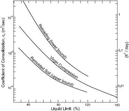
Because of the wide range of permeabilities that exist in soils (see Table 1-10), the coefficient of consolidation can itself vary widely, from less than 10 ft²/yr (≈1 m2/yr) for clays of low permeability to 10,000 ft²/yr (≈1,000 m²/yr) or more for very sandy clays, fissured clays and weathered rocks. Some typical values for clays are given in Table 1-6 and an approximate correlation with liquid limit is shown in Figure 1-10.

Just as permeabilities in the horizontal and vertical directions can be significantly different due to variations in soil particle orientation, non-homogeneity, etc., so too can the in situ coefficient of horizontal consolidation, c_h, be much different from the coefficient of vertical consolidation cv measured in the laboratory for the same reasons. For example, the in situ coefficient of horizontal consolidation, c_h, for clays containing fissures or fine bands of sand, may often be much greater than cv measured in the laboratory for the clay alone. In such cases, the in-situ c_h may govern the actual rate of consolidation under field loading conditions.

1.4.6.4 Coefficient of Secondary Compression, C_α

Table 1-7 presents typical values of C_α in terms of Cc for various geomaterials. As shown below by Equations 1-7, the coefficient, C_α, may be expressed either in units of strain (C_αε) or void ratio (C_αe) per log cycle of time. As indicated previously, to convert void-ratio-based consolidation curve indices to strain-based indices divide the void-ratio-based values by (1 + e_o).

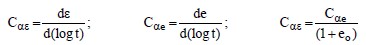
C_αe is usually assumed to be related to Cc with values of C_αe/C_c typically in the range 0.0250.006 for inorganic soils and 0.035-0.085 for organic soils. Figure 1-11 presents a correlation between C_αe and natural water content.

1.5 Shear Strength of Soils

The shear strength of soils is extremely important to foundation design. In addition, slopes of all kinds, including hills, river banks, and man-made cuts and fills, stay in place only because of the shear strength of the material of which they are composed. Knowledge of the shear strength of soil is important for the design of structural foundations, embankments, retaining walls, pavements, and cuts. Table 1-8 provides a summary of specific issues related to the design and construction of typical highway design elements that should be considered in developing and implementing a laboratory and in-situ testing program for evaluating soil shear strength.

1.5.1 Concept of Frictional and Cohesive Strengths

The concept of shear strength was shown to be comprised of two components, friction (φ) and cohesion (c). In terms of the classification of soils, these two components of the shear strength can be generalized as follows:

1. Coarse-grained soils, such as gravel and sand, and fine-grained silt, derive strength primarily from friction between particles. Therefore they are considered to be “cohesion less” or “frictional” soils and are often denoted as “φ-soils.”
2. Fine-grained soils, composed mainly of clay, derive strength primarily from the electro-chemical attraction, or bond, between particles. Therefore they are considered to be “cohesive” soils and are often denoted as “c-soils.”
3. Mixtures of cohesion less and cohesive soils derive strength from both interparticle friction and bonding. Such soils are commonly denoted as “c-φ soils.”

1.5.1.1 Strength Due to Friction

The strength due to friction between soil particles is dependent on the stress state of the soil (e.g., overburden pressure) and the angle of internal friction (φ) between the particles. The frictional resistance of soil is equal to the normal stress, σn, times the tangent of friction angle, φ. The tangent of φ is equal to the coefficient of friction (μ) between the soil particles.

The equation for frictional resistance, τ, is written in terms of normal stress, σ_n, as follows:

The coefficient of friction, tan φ, between individual particles depends on both their mineral hardness and surface roughness. However, the measured friction angle of a soil sample or deposit also depends on the density of the mass caused by interlocking of particles. For a detailed discussion of factors affecting frictional resistance, the reader is referred to textbooks such as by Holtz and Kovacs (1981).

1.5.1.2 Strength Due to Cohesion

The concept of cohesive strength is more difficult to explain and often misunderstood. The designer must develop a good understanding of this concept otherwise there will be a disconnect between reality and the design of some structures, e.g., the first bench cut in shoring.

There are two types of cohesion in soils: true cohesion and apparent cohesion. These are briefly discussed as follows (after Mitchell, 1976):

1. True cohesion may result from chemical cementation (just like in rocks) and/or forces of attraction (e.g., electrostatic and electromagnetic attractions) between colloidal (10^-3 mm to 10^-6 mm) clay particles. True cohesion is stress-independentunlike frictional resistance that is a function of normal stress.
2. Apparent cohesion may develop because of capillary stresses and mechanical interlocking as follows:

• Capillary stresses develop between particles in a partially saturated soil due to surface tension in the water. The surface tension (negative pressure) in the water produces an equal and opposite effective stress between the soil particles, which results in an apparent cohesion since it too is stress-independent. The magnitude of this type of apparent cohesion can be extremely large, especially in fine-grained soils. Such capillary stresses can be overcome by an increase in the degree of saturation.
• Apparent mechanical forces are often exhibited by the interlocking of rough(angular) soil particles. The interlock between the soil particles can offer some resistance to shear stresses even in the absence of a normal stress. This type of apparent cohesion is often the cause of cohesion measured in compacted soils. However, such apparent mechanical forces are susceptible to significant reduction by vibrations and other types of mechanical disturbance.

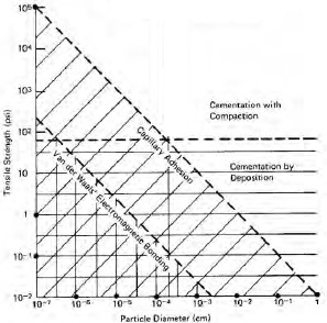
Figure 1-12 presents a graphical representation of the potential contribution of various mechanisms of cohesion. It can be seen that true cohesion in soils exists only when the particle size is colloidal. Unless the complete soil sample is composed of colloidal particles, true cohesion due to interparticle attraction cannot be relied on. Cementation by deposition is often observed in arid environments (e.g., desert southwest), but it is difficult to quantify. As indicated above, capillary stresses can provide a large apparent cohesion, but such cohesion can be overcome by saturation. Since cohesion cannot be defined with confidence, its contribution to long-term shear strength in c-φ soils is often disregarded or greatly minimized by using only a small value such as 100 to 500 psf (5 to 25 kPa). For purely cohesive soils, the designer should be careful in evaluating the cohesion for long-term design purposes. Further discussion on apparent cohesion in the context of compacted soils is included in Section 1.8.4.1.

1.5.1.3 Simplified Expression for Shear Strength of Soils

The shear strength, τ, of soils is expressed simplistically by two additive components as follows:

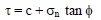
In terms of effective stresses, the effective shear strength, τ′, can be re-written as follows:

where u is the pore water pressure, c′ is the effective cohesion, σ′ is the effective normal stress, and φ′ is the effective friction angle.

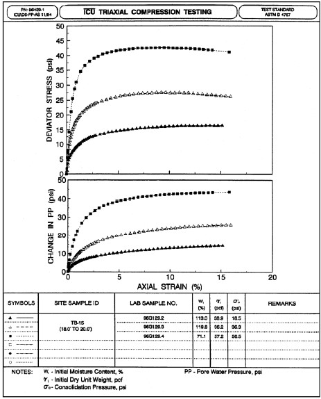
The shear strength soil is influenced by many factors including the effective stress state, mineralogy, packing arrangement of the soil particles, soil hydraulic conductivity, rate of loading, stress history, sensitivity, and other variables. As a result, the shear strength of soil is not a unique property. The following sections present and discuss various laboratory tests to determine the shear strength for various types of construction and loading conditions. Typical laboratory strength tests are introduced including the unconfined compression test (AASHTO T208; ASTM D 2166), the triaxial test (AASHTO T234; ASTM D 4767), and the direct shear test (AASHTO T236; ASTM D 3080). A detailed discussion on testing equipment and procedures is beyond the scope of this document. The interested reader should review the AASHTO and ASTM standards for detailed information on testing equipment and procedures. The following sections also describe information that must be conveyed to a laboratory testing firm to ensure that the strength testing is performed consistent with the requirements imposed by the design (e.g., selection of confining pressures consistent with the imposed loads).

1.5.2 Strength Testing of Soils in the Laboratory

The shear strength of a soil is the maximum shear stress that the soil structure can resist before failure. Failure is generally defined as continuing displacement without an increase in applied stress. Since the water filling the pores has no shear strength, shear stresses are carried by the structure of soil grains. However, the shear strength of the soil structure is indirectly dependent on the pressure in the pore water, which influences the friction term as shown by the excess pore water pressure term, u, in Equation 1-10. Foundation designers must consider the effects of expected construction operations on the subsoils when planning a test program. For example, when a highway embankment or structural footing is suddenly placed on a soft clay deposit, the pore water initially carries all the load and the available shear strength does not increase until drainage begins and the excess pore water pressure decreases. In planning a test program for such a situation the designer should request unconsolidated undrained (UU) triaxial tests to determine the undrained shear strength of the soil which, in this case, would be the critical strength value, i.e., the initial shear strength before consolidation begins. Additional consolidated undrained (CU) or consolidated drained (CD) tests would also be used to determine the increase in shear strength as consolidation occurs and excess pore water pressures dissipate. These results can be used to determine alternate methods of applying the loads safely, especially if the undrained strength is insufficient to sustain the proposed loading. Stage construction involves placement of an increment of load and a waiting period to allow strength gain through excess pore water pressure dissipation so the soil deposit can safely support the next load increment.

The majority of strength tests are conducted on cohesive soils since obtaining undisturbed samples of non-cohesive soils is difficult. Strength tests on cohesive soils are usually conducted on high quality undisturbed samples obtained from thin wall sampling tubes. The preferred test for most projects where cohesive soils are involved is the triaxial compression test. The number and types of tests must be selected by the designer to suit the project conditions. For each test the designer should clearly indicate the consolidation or confining pressure to be used. These pressures are determined from the po diagram for each specific project. The range usually extends from the effective overburden pressure to the pressure induced by the highway loading. The program objective should be to establish a profile of soil strength with depth. Soil strength parameters are frequently expressed as a ratio of shear strength over the effective overburden pressure (τ/p_o).

The most common laboratory soil strength tests are:

• Unconfined compression test
• Triaxial compression test, and
• Direct shear test

Each of these tests is briefly discussed below. For the triaxial compression and the direct shear tests, it is important that each test be performed on a new sample. The practice of performing multi-stage shear strength tests on a single sample is not recommended.

1.5.2.1 Unconfined Compression (UC) Tests

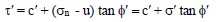
The unconfined compression test is a quick, relatively inexpensive means to obtain an estimation of the undrained shear strength of cohesive specimens. In this test a cylindrical specimen of the soil is loaded axially as shown in Figure 1-13 without any lateral confinement to the specimen, at a sufficiently high rate to prevent drainage. Since there is no confinement, residual negative pore pressures that may exist in the sample following sample preparation generally control the state of effective stress in the sample. The shear stresses induced in the specimen by the axial load result in a shear failure. The magnitude of the shear stress at the moment of failure represents the shear strength of the soil under these conditions of loading and drainage. Therefore, the shear strength obtained from this test is called the “undrained shear strength (s_u).” In most cases, the value of undrained shear strength obtained from an unconfined compression test is conservative. The maximum axial compressive stress measured at failure represents the compressive strength of the soil under these conditions of loading, drainage, and confinement. Therefore, the compressive strength obtained from this test is called the “unconfined compressive strength (q_u).” These two strengths terms should not be confused; one is a shear strength the other a compressive strength. It can be shown graphically by a Mohr’s circle construction (Appendix B) that the undrained shear strength (s_u) is equal to one-half the unconfined compressive strength (q_u).

The unconfined compression test cannot be performed on granular soils, dry or crumbly soils, silts, peat, or fissured or varved materials. Because there is no control over the effective stress state of the specimen, this test is not recommended for evaluating strength properties for compressible clay soils subjected to embankment or structural foundation loads. The reliability of this test decreases with increasing sampling depth because the sample tends to swell after removal from the ground due to confining stress release. The swelling results in greater particle separation and reduced shear strength. Testing the full diameter extruded specimen as soon as possible after removal from the tube can:

• minimize swelling
• reduce disturbance
• preserve the natural moisture content.

Unfortunately, despite these shortcomings, this test is commonly used in practice because of its simplicity and low cost.

1.5.2.2 Triaxial Tests

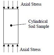
The triaxial test is very versatile in the sense that the shear strength can be evaluated under compression as well as extension loading conditions. A schematic of triaxial compression test is shown in Figure 1-14 where the axial stress is greater than the confining stress. Lateral pressures at various depths below the ground surface can be simulated by confining pressures. Note that the confining pressures acts on the entire sample and is equal to the axial stress before the application of an axial stress increment. Typically, failure of the sample is caused by increasing the axial stress (compression) until a shear failure takes place. In an extension test, the confining pressures are increased while keeping the axial stress constant. Pore water pressures during the test can be measured.

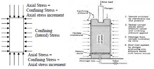
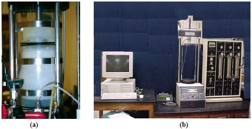
Equipment – Triaxial systems today use electronic instrumentation to provide continuous monitoring and periodic acquisition of test data (see Figure 1-15b). Force is measured by using a force transducer or load cell that is typically mounted outside the triaxial cell. More advanced systems have the transducer incorporated within the testing cell to reduce the effects of rod-friction. Linear variable differential transducers (LVDTs) are used to monitor deformations. Additionally, volume measurements can be taken with a device that makes use of an LVDT to measure the rise or fall of a bellofram cylinder. This change in movement is calibrated to the volume of water taken in or pushed out of the sample. Pressure transducers are mounted on the base of the test cell to monitor the confining pressure within the cell and the pore water pressure within the sample.

Unconsolidated-Undrained (UU) Test

In the UU test, no drainage or consolidation is allowed during either the application of the confining pressure or the application of the axial load that induces shear stress. The shear stresses induced in the specimen by the axial load result in failure. As indicated in Section 1.5.2, the UU test models the response of a soil that has been subjected to a rapid application of an axial load such as that due to construction of an embankment. It is difficult to obtain repeatable results for UU testing due to the effects of sample disturbance. The accuracy of the UU test is dependent on the soil sample retaining its original structure until testing occurs. The undrained shear strength of the soil, s_u, is measured in this test.

Consolidated-Drained (CD) Test

In the CD test, the specimen is allowed to consolidate completely under the confining pressure prior to the application of axial load, i.e., the confining pressure acts as an effective stress throughout the soil specimen. The axial load is applied at a rate slow enough to allow drainage of pore water so that there is no buildup of excess pore water pressures, i.e., the stresses imposed by the axial load are effective stresses. The shear stresses induced in the specimen by the axial load result in failure. The time required to conduct this test in low permeability soil may be as long as several months. Therefore it is not common to conduct a CD test on low permeability soils. The CD test models the long-term (drained) condition in soil. Effective stress strength parameters (i.e., φ′ and c′) are evaluated from the results of the CD test.

Consolidated-Undrained (CU) Test

The initial part of the CU test is similar to the CD test in that the specimen is allowed to consolidate under the confining pressure. However, unlike the CD test, the axial load is applied with the drainage lines closed in the CU test. Thus, during shearing there is continual development (+ or -) of excess pore water pressure. The rate of axial load application for this test is more rapid than that for a CD test. Pore pressures are typically measured during the CU test so that both total stress and effective stress strength parameters can be obtained. Recall that total stress equals effective stress + pore water pressure as expressed by Equation 1-13. The pore water pressure may be + or – depending upon whether the specimen dilates or compresses during application of the axial load. The shear stresses induced in the specimen by the axial load result in failure. The effective stress parameters evaluated for most soils based on CU testing with excess pore water pressure measurements will be similar to those obtained from CD testing, thus making CD tests unnecessary for typical applications.

During triaxial testing, the confining pressure, which acts uniformly over the entire specimen, is considered to be the minor principal stress. By definition, a principal stress is one that acts on a plane where shear stress is zero. The interface between the soil and the membrane isolating it from the fluid in the chamber is assumed to be frictionless during the entire test, i.e. no shear stresses develop along the circumference of the specimen. Likewise, the applied axial load causes a normal stress to act on the top and bottom of the specimen. As shown in Figure 1-14, this vertical normal stress acts in addition to the confining pressure. Therefore, the combined vertical stress acting on the top and bottom of the specimen during the triaxial test is considered to be the major principal stress not only because the plane (horizontal) on which it acts is orthogonal to the minor principal stress plane (vertical), but mainly because the interface shear stress between the specimen and the top and bottom caps is assumed to be equal to or close to zero. To assure this condition, the end caps are usually coated with a lubricant to make them virtually frictionless. Because of these boundary stress conditions, the specimen is free to shear on a plane consistent with the directions of the major and minor principal stress planes and its inherent shear strength as expressed by c and φ.

1.5.2.3 Direct Shear Tests

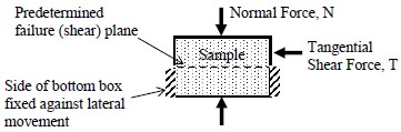
The oldest form of shear test upon soil is the direct shear test, first used by Coulomb (1776). A schematic of the essential elements of the direct shear apparatus are shown in Figure 1-17. The soil is held in a box that is split across its middle; the bottom portion of the box is usually fixed against lateral movement. A confining normal force, N, is applied, and then a tangential shear force, T, is applied so as to cause relative displacement between the two parts of the box. The magnitude of the shear force is recorded as a function of the shear displacement, and usually, the change in thickness of the soil sample is also recorded. Although it is widely used in practice, the direct shear device lacks a number of features that limit is applicability. For example, there is no way to control the confining pressure. Also, since there is no way to measure excess pore water pressures generated during shearing of saturated clay specimens, use of the direct shear test is generally limited to cohesionless soils.

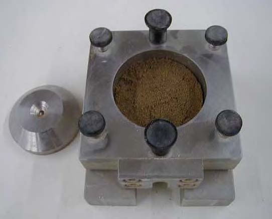
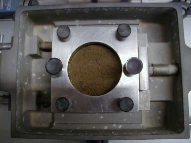
Equipment – The apparatus and procedures for direct shear testing are discussed in ASTM D 3080. A specimen is prepared in a split square or circular box. Figure 1-18 shows a circular specimen. The specimen is sheared as one part of the box is displaced horizontally with respect to the other. Generally, the lower part of the box is fixed against lateral movement and the shear force is applied to the upper part of the box through a loading frame as shown in Figure 1-18. The central two of the six screws visible in the top portion of the box extend into the bottom portion and are used to hold the assembly together while the specimen is being prepared. This shear box assembly is then placed in a reservoir which could be filled with water to allow saturation of the specimen prior to shearing. Before the test is begun, the two central screws are removed and the four corner screws, which rest on the top surface of the bottom portion of the box, are turned to slightly raise the top part of the box so that there is no contact between it and the bottom part of the box. This is done to prevent the error that would result from the frictional resistance between the two boxes at their contact. Load cells are used to monitor the shear force and LVDTs are used to monitor both horizontal and vertical deformation. By use of this instrumentation, as well as a loading frame that provides a constant rate of horizontal deformation, it is possible to automate the direct shear test.

Test Procedures – In the direct shear test, the soil is first consolidated under an applied normal stress. After consolidation is completed, which will be virtually instantaneous in cohesionless soils, the specimen is sheared directly at a constant rate. The rate of shear is typically selected as a function of the hydraulic conductivity of the specimen. Direct shear testing is commonly performed on compacted materials used for embankment fills and retaining structures. Direct shear testing can also be performed on natural materials. However, the lack of control on soil specimen drainage makes the evaluation of undrained strength unreliable. The direct shear test can also be used to evaluate the drained strength of natural materials by shearing the sample at a rate slow enough to ensure that no significant pore water pressures develop, however there is no way to verify this condition by measurement.

In addition to providing data that allows the determination of the peak effective stress friction angle (φ′), the direct shear test data can also be used for the evaluation of effective stress residual strengths (c′_r ≈ 0; φ′_r). The effective stress residual strength parameters are necessary for stability and landslide analyses. Residual strengths are associated with very large shear strains along a predefined or preferential slip surfaces that result in very large deformations. Data from a reversing direct shear test can also be used to evaluate residual shear strengths. In a reversing direct shear test, the direction of shearing in the test is reversed several times thereby causing the accumulation of displacements at the slip surface.

A characteristic of the direct shear test that distinguishes it from the triaxial test is that the shear failure in the direct shear device is forced to occur on a horizontal plane so that the orientations of the major and minor principal stress planes are not apparent. Ordinarily this characteristic is considered to be a disadvantage of the direct shear test. However this characteristic is advantageous for designs involving geosynthetics where the shearing resistance of the interface between the soil and the geosynthetic or between two pieces of geosynthetic is often required. Direct shear machines have been modified to test the interface shear strength between various types of engineering materials, as described in ASTM D 5321.

1.5.3 Factors Affecting Strength Testing Results

It is important for the designer to realize that all laboratory tests on soils must be carefully performed. This is particularly important for strength testing since the use of strength parameters are a key to successful foundation design. The following seven factors in particular affect the results of strength testing:

1. Sample disturbance
2. Mode of shearing
3. Confining pressures
4. Specimen size
5. Saturation
6. Displacement at failure
7. Rate of shearing and strain required to reach peak strength

A detailed discussion of each of these factors is presented in FHWA (2002a). In addition to recognizing the effect of the factors that can affect the strength testing results, it is extremely important for the designer to perform the proper tests depending on project requirements. The selection of an appropriate test to be used to provide relevant information for a particular geotechnical structure should consider, at a minimum, the following questions:

1. How fast will construction occur relative to the hydraulic conductivity of the soil(i.e., should drained or undrained strength tests be performed)?
2. How does the direction of applied load affect measured shear strengths and the appropriate strength to be used for an analysis?
3. How do the expected levels of deformation for the geotechnical structure affect the selection of shear strength? and
4. How does the manner in which the feature is constructed affect the shear strength to be used in analysis?

1.5.4 Comparison of Laboratory and Field Strengths

Soil samples are obtained from the ground for laboratory testing by sampling from boreholes and sealing and transporting these samples to the laboratory. The degree of disturbance affecting the samples will vary according to the type of soil, sampling method and the skill of the driller. At best some disturbance will occur from the removal of in-situ stresses during sampling and from the preparation of specimens in the laboratory for testing. In general, disturbance tends to reduce the shear strength obtained from unconfined or unconsolidated tests and increase the shear strength obtained from consolidated tests. There is, therefore, considerable merit in measuring the in-situ shear strength. The field vane shear test is the most commonly used field test for direct measurement of the undrained shear strength of soft to medium clays. In reviewing the different types of field and laboratory tests available to determine the undrained shear strength in clays, the designer should expect the field vane shear test to provide the most accurate value of s_u, with UC and UU tests yielding lower results and CU tests yielding slightly higher results.

It is important that the results of in-situ tests be interpreted carefully and calibrated with laboratory tests. Without careful calibrations, the in-situ tests can yield inaccurate results.

1.5.5 Selection of Design Shear Strength

Frequently, on a large project the designer will receive a large quantity of undrained shear strength test results from both the field and laboratory. This data must be synthesized to permit rational interpretation of the results. The tests should be analyzed on a hole-by-hole basis. All tests from one hole should be reviewed and the results for each type of test should be plotted separately versus depth to determine the pattern of strength variation for each test type and to assess the reliability of the data, e.g., a CU test result that is lower than a UC test result at the same depth should be considered suspect. The general pattern of shear strength results should show an increase in strength with depth in a normally consolidated clay deposit. Overconsolidated clays may exhibit this pattern only at greater depths since the amount of preconsolidation increases shear strength in the upper portions of the soil deposit. Section 1.14 presents values of the coefficient of variation of measured soil properties that should be taken into account while selecting the final design shear strength.

1.5.6 Correlations of Shear Strength Parameters with Index Parameters

This section presents some useful correlations between shear strength parameters and other index values or field conditions. These correlations may be used by the designer to check the general validity of the laboratory test results or to develop a preliminary assessment about the shear strength characteristics of the soils on the project site. In the latter case, it must be emphasized that predictions based on correlations alone should never be used for design and that any assumptions regarding shear strength parameters must always be verified through testing.

1.5.6.1 Undrained Shear Strength of Cohesive Soils

For most saturated clays tested under quick undrained conditions, the angle of shearing resistance, φu, is zero. This means that the shear strength of the clay is a fixed value and is equal to the apparent cohesion, cu, at a specific moisture content and preconsolidation pressure. A value for the undrained shear strength may be crudely estimated for a sample for which uncorrected SPT N-values are known by molding a specimen of the clay between the fingers and by applying the observations indicated. However, the values of SPT blow count listed there should not be used to determine the design strength of fine grained soils.

Undrained Shear Strength

For most normally consolidated clays the undrained shear strength (s_u) is proportional to the effective overburden pressure (p_o). For such soils, Skempton (1957) proposed the relationship shown in Figure 1-20 between the s_u/p_o and plasticity index (PI). Figure 1-20 also includes results obtained by a number of other researchers. As can be seen in the figure, the composite of all findings varies so much that such relations should be used with caution. However, such correlations, particularly the correlation by Skempton (1957), are useful for obtaining preliminary estimates and for checking laboratory results of project-specific tests performed on normally consolidated clays.

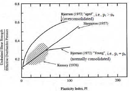
The shear strength of undisturbed clays depends on the consolidation history of the clay as well as its fabric characteristics. In general, the undrained strength ratio, su/po, increases with increasing overconsolidation as measured by the overconsolidation ratio, OCR. It is recommended that laboratory tests be performed to determine the undrained strength ratio for overconsolidated clays rather than relying on any published correlations. In practical terms, it is more straightforward to measure the undrained shear strength of overconsolidated clays than to predict it from other indices.

1.5.6.2 Drained and Effective Shear Strength of Cohesive Soils

It is often important to carry out stability calculations in terms of effective stresses. The soil strength parameters, c′ and φ′, used in these calculations should be obtained from either drained direct shear box or drained triaxial tests or from CU triaxial tests with pore water pressure measurements (giving φ′_cu and c′_cu). Generally, there is a minor difference in the results obtained from these two tests for saturated clays because the soil is being tested under different boundary conditions and stress paths. In-situ tests such as CPTs can also be used to estimate the drained and effective shear strength parameters of cohesive soils.

For clays, empirical correlations have been developed to relate φ′ to the plasticity characteristics of the soil. Figure 1-21 shows a slight trend of φ′ decreasing with increasing PI. The existence of these relationships arises because both PI and shear strength reflect the clay mineral composition of the soil; as the clay mineral content increases, the PI increases and the strength decreases. From Figure 1-21, it can be seen that the drained friction angle values can be ± 8° in variance with respect to the dashed trend line.

Considering the overall importance of φ′ in stability calculations, foundations design, and landslide analyses, it is essential to assess φ′ directly by means of consolidated drained direct shear tests, consolidated drained triaxial tests, or consolidated undrained triaxial tests with pore water pressure measurements. The consequences of merely estimating φ′ can be economically unwise. As an example, in stability analyses for relatively long, shallow slip surfaces that may be associated with a landslide, the required forces that would need to be resisted by some form of stabilization system (e.g., retaining wall, micropiles) would vary significantly depending on the drained friction angle of the soil. It is highly recommended that geotechnical designers develop historical data summaries of φ′ versus PI to check the validity of future test results.

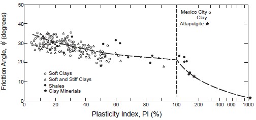
1.5.6.3 Shear Strength of Cohesionless Soils

Because of their high permeability, pore water pressures do not build up significantly when cohesionless soils are subjected to shearing forces. The complication of total and effective stresses is therefore avoided and the phenomenon of apparent cohesion, or undrained shear strength does not occur. Consequently, the shear strength of cohesionless soils is defined exclusively in terms of frictional resistance between the grains, as measured by the angle of shearing resistance, φ. Typical values of φ for sands and gravels are given in Figure 1-22 as a function of dry unit weight and relative density. The material types indicated in the figure relate to the Unified Classification System (USCS).

Figure 1-22 requires determination of relative density. A reasonable estimate of relative density can be obtained from Figure 1-23. Figure 1-23 was originally developed based on data obtained using rope and cathead operated hammers. Thus, it is recommended that an energy corrected SPT N-value, i.e., N₆₀, be used as shown in Figure 1-23. However, note that Figure 1-23 is a function of both N-value and the vertical effective overburden pressure, p_o. Therefore, N60-value should not be corrected for overburden pressure, i.e., C_N=1.0 while using Figure 1-23.

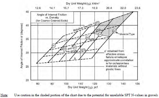
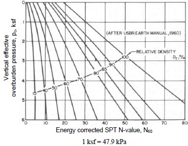
1.6 Permeability

1.6.1 General

Permeability, also known as hydraulic conductivity, is one of the major parameters used in selecting soils for various types of construction. In some cases, it may be desirable to place a high-permeability fill immediately under a pavement surface or behind a wall to facilitate the removal of water. In other cases, such as retention pond dikes, it may be detrimental to use high-permeability materials. Permeability also significantly influences the choice of backfill materials for various elements such as trenches and retaining walls.

Unlike the fill soils discussed in the previous paragraph, the permeability of a natural soil is strongly influenced by its macroscopic structure, e.g., clays containing fissures or fine bands of sand will have permeabilities that are many times greater than that of the clay material itself. Also, stratified soils often have horizontal permeabilities that are many times the vertical permeability. Because of the small size of laboratory specimens and the way they are obtained and prepared, large scale in-situ features are absent and test results do not give a true indication of field values in soils with a pronounced macro-structure. Moreover, laboratory tests usually constrain water to flow vertically through the specimen whereas the horizontal permeability may be much greater, and hence of overriding importance, so far as site conditions are concerned. Field permeability tests overcome these shortcomings, but, since the pattern of water flow from a well used to determine in situ permeabilities can only be estimated, interpretation of the field test results is difficult and uncertain. Thus, one set of problems is exchanged for another.

1.6.2 Equipment

Laboratory permeability testing is performed to determine the permeability or hydraulic conductivity (k) of a soil specimen. For natural soils, tests are conducted on specimens from tube samples. For fill and borrow soils, tests are performed on compacted materials. Two types of tests are commonly performed, the rigid wall test (AASHTO T215; ASTM D 2434) and the flexible wall test (ASTM D 5084).

The equipment for the rigid wall test includes a rigid wall permeameter, a water tank, a vacuum pump, and manometer tubes (see Figure 1-24). The permeameter must be large enough to minimize sidewall leakage. Therefore, the diameter of the rigid wall device should be at least 8 to 12 times that of the largest soil particle in the sample being tested. Frequently, the side wall of the cylinder is coated with petroleum jelly to prevent sidewall leakage. Porous stones and filter paper placed on the top and bottom of the test specimen to prevent soil particle erosion by retaining fine particles must not restrict flow through the soil otherwise the permeability of the porous stones or filter paper will be measured. A vacuum pump is used to remove air from the sample and to help saturate the specimen prior to testing. In a rigid wall test saturation is performed from the bottom of the specimen upward (see ASTM D 2434). Manometer outlets should be available on the sides of the cell to measure head loss over the specimen.

Rigid wall permeameters are not recommended for low permeability (i.e., k ≤ 2 x 10^-5 ft/min (1 x 10^-6 cm/s)) soils due to the potential for sidewall leakage. Rigid wall permeameters are typically used for sandy and gravelly soils (ASTM D 2434) with a permeability greater than 2×10^-2 ft/min (1×10^-3 cm/s). Rigid wall systems are used for granular materials because the permeability of the flexible wall system (valves, pore stones, tubing, etc.) may be less than that of the specimen. Therefore the flexible wall system itself may affect the permeability value of granular soils and a measured value of permeability lower than that of the specimen may result.

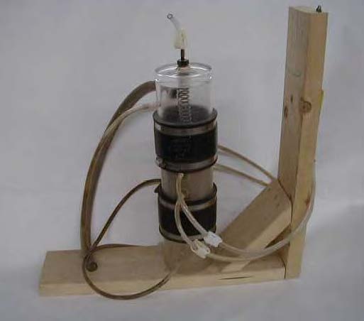
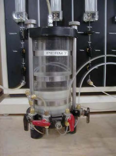
The equipment for a flexible wall test includes a flexible wall permeameter cell, a cell reservoir, a headwater reservoir, a tailwater reservoir, top and base caps, a flexible membrane, porous stones, and filter paper (see Figure 1-25). The specimen can be tested over a range of confining stresses under backpressure saturation. The separate headwater and tailwater reservoirs can be monitored, and falling head or constant head tests can be performed. Since the flexible membrane encases the specimen, side leakage is prevented. Flexible wall permeameter cells consist of influent and effluent lines as well as porous stones and filter paper. The hydraulic conductivity of the system should be tested before a soil specimen is tested to ensure that the system’s conductivity is at least one order of magnitude greater than that anticipated for the soil. The triaxial cell can be used as a flexible wall permeameter. In fact, permeability measurements are often made as part of a drained triaxial (CD) test.

The determination of permeability by testing is predicated on the validity of Darcy’s Law for laminar flow through porous media. If any of the assumptions of Darcy’s Law are violated, the results of permeability testing will be invalid.

1.6.3 Procedures

Flexible wall permeameters (ASTM D 5084) are used for materials with a hydraulic conductivity (k) less than or equal to 2×10^-2 ft/min (1×10^-3 cm/sec). The flexible membrane used to encase the specimen prevents sidewall leakage for fine-grained soils that are likely to occur in a rigid wall system. The confining stress of the hydraulic conductivity test should be specified to the laboratory. As confining stress increases, the hydraulic conductivity of fine grained soils will typically decrease due to consolidation of the specimen and reduction of void ratio. The confining stress should be equal to the anticipated effective stress-state in the soil.

The hydraulic gradient, defined as the difference in hydraulic head across the specimen divided by the length of the specimen, should also be specified to the laboratory. Typical hydraulic gradients in field situations are less than 5, however the use of such a small gradient in the laboratory will result in extremely long testing times for materials having hydraulic conductivities less than 2×10^-5 ft/min (1×10^-6 cm/sec). If the hydraulic gradient across the specimen is too high, turbulent flow will occur and Darcy’s Law will be violated with the result that the measured hydraulic conductivity will be less than that which will occur in the field. Suggested values of hydraulic gradient, as presented in Table 1-9, are a function of the anticipated hydraulic conductivity.

Saturation of the specimen is necessary to achieve accurate results. A hydraulic conductivity test should be ended when steady flow is occurring. The flow through the permeameter is considered to be steady when four or more consecutive hydraulic conductivity measurements fall within ±25 percent of the average k value if k is greater than 1 x 10^-8 cm/sec, or if four or more measurements fall within ±50 percent of the average if k is less than 1 x 10^-8 cm/sec.

1.6.4 Useful Correlations of Permeability with Index Values

The typical range of permeability values for various soil types and USCS groups is presented in Table 1-10, which is based on information originally presented by Casagrande and Fadum (1940). Superimposed on Table 1-10 are “typical soil groups” identified by their USCS symbols (Carter and Bentley, 1991). The range of permeability values corresponding to those groups is typical for compacted soils of that type where compaction is according to ASTM D 1557. Typical permeability values for highway construction materials are given in Table 1-11.

Numerous correlations of permeability with grain size can be found in the literature. Figure 1-26 presents logarithmic plots of k versus D10, based on experimental results. Figure 1-26 includes the well known Hazen’s formula. All the correlations shown in Figure 1-26 were developed for sands and gravels. The great range of particle size present in most clays and the effects of clay mineralogy make such correlations of limited use for clays.

Hazen’s equation is the most common correlation equation used to estimate permeability for sands (k > 10^-3 cm/sec). This equation is written as:

where: k is the permeability in cm/s;

• C = a coefficient ranging from 0.4 to 1.2 depending on sand size/sorting; and
• D10 = effective grain size in mm at 10% passing by weight as determined from sieve analysis.

Hazen’s equation should be used with caution since it provides very approximate estimates of k applicable only to clean sands having less than 5% passing the No. 200 sieve (0.075 mm)and with D10 sizes between 0.1 and 3.0 mm (Holtz and Kovacs, 1981). Hazen’sequation is valid only for k > 10^-3 cm/sec.

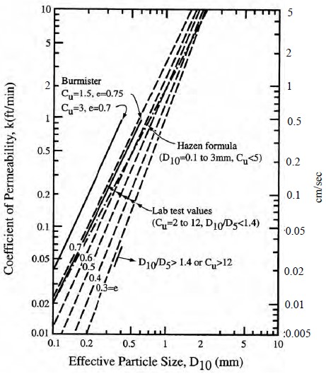
Note: in Figure 1-26, correlations shown are for remolded compacted sands and sand-gravel mixtures with C_u values as indicated.

1.7 Volume Change Phenomena Due to Loading and Moisture

Depending on mineralogy and depositional patterns, natural soils can exhibit either swell (expansion) or collapse under various degrees of loading and moisture ingress. Moisture may be in liquid or frozen form. For foundation design, it is very important to recognize and evaluate the potential for soils to swell or collapse. It is important to realize that these phenomena happen in both natural and compacted soils. Every year millions of dollars are spent dealing with the consequences of swelling (expanding) and collapsing soils. This section briefly discusses these two mechanisms and the tests that can be performed to evaluate the swell (expansion) and collapse potentials.

1.7.1 Swell Potential of Clays

Swelling is a characteristic reaction of some clays to water ingress. The potential for swell depends on the mineralogical composition of the soil fines. While montmorillonite (smectite) exhibits a high degree of swell potential, illite has no to moderate swell potential, and kaolinite exhibits almost none. The percentage of volumetric swell of a soil depends on the amount and type of clay, its relative density, the compaction moisture content and dry density, permeability, location of the groundwater table, the presence of vegetation and trees, overburden pressure, etc. Expansive soils are found throughout the U.S., however, damage caused by expansive clays is most prevalent in certain parts of California, Wyoming, Colorado, and Texas, where the climate is considered to be semi-arid and periods of intense rainfall are followed by long periods of drought. This pattern of wet and dry cycles results in periods of extensive near-surface drying and desiccation crack formation. During intense precipitation, water enters the deep cracks causing the soil to swell; upon drying, the soil will shrink. This weather pattern results in cycles of swelling and shrinking that can be detrimental to the performance of pavements, slabs on-grade, and retaining walls built on or in such soils.

Deep-seated volume changes in expansive soils are rare. More common are volume changes within the upper 3-10 feet (1- 3 m) of a soil deposit. These upper few feet are more likely to be affected by seasonal moisture content changes due to climatic changes. The zone over which volume changes are most likely to occur is defined as the active zone. The active zone can be evaluated by plotting the moisture content with depth for samples taken during the wet season and for samples taken during the dry season at the same location. The depth at which the moisture content becomes nearly constant is the limit of the active zone depth, which is also referred to as the depth of seasonal moisture change. The active zone is an important consideration in foundation design. In the design of piles or drilled shafts, it is important to recognize that full side friction resistance may not be realized in this zone. As the soil undergoes cycles of shrinking and swelling, it may lose contact with the pile or shaft. Alternatively, as the soil swells, it may impose significant uplift pressures on the foundation element.

In the field, the presence of surface desiccation cracks and/or fissures in a clay deposit is an indication of expansion potential. Experience has indicated that the most problematic expansive near-surface soils are typically highly plastic, stiff, fissured, overconsolidated clays. Several classification methods are used to identify expansive soils in the laboratory. Currently, there is not a standard classification procedure; different methods are used in various locations across the U.S. Typically, methods include the use of Atterberg limits and/or clay size percentage to describe a soil qualitatively as having low, medium, high, or very high expansion potential. Generally, soils with a plasticity index less than 15 percent will not exhibit expansive behavior. For soils with a plasticity index greater than 15 percent, the clay content of the soil should be evaluated in addition to the Atterberg limits. Figure 127 shows the swelling potential of natural soils and soils compacted to standard Proctor procedures (ASTM D 698) as a function of modified activity index, Am, (Equation 1-4) and clay fraction.

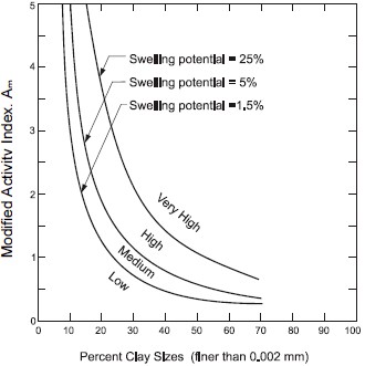
1.7.1.1 Evaluation of Expansion (Swell) Potential

For situations where it is necessary to construct a facility in and around expansive soils, it will be necessary to estimate the magnitude of swell, i.e., surface heave, and the corresponding swelling pressures that may occur if the soil becomes wetted. The swelling pressure represents the magnitude of pressure that would be necessary to resist the tendency of the soil to swell. A one-dimensional swell potential test can be performed in an oedometer on undisturbed or recompacted samples according to AASHTO T256 or ASTM D 4546. In this test, the swell potential is evaluated by observing and measuring the swell of a laterally confined specimen when it is lightly surcharged and flooded with water. Alternatively, if the swelling pressure is to be measured, the height of the specimen is kept constant by adding load after the specimen is inundated. The swelling pressure is then defined as the vertical pressure necessary to maintain zero volume change. Swelling pressures in some expansive soils may be so large that the loads imposed by lightweight structures or pavements do little to counteract the swelling.

The use of the one-dimensional swell potential test to evaluate in-situ swell potential of natural and compacted clay soils has limitations including:

• Lateral swell and lateral confining pressure are not simulated in the laboratory. The calculated magnitude of swell in the vertical direction may not be a reliable estimate of soil expansion for structures that are not confined laterally (e.g., bridge abutments);
• The rate of swell calculated in the laboratory will not likely be indicative of the rate of swell experienced in the field. Laboratory tests cannot simulate the actual availability of water in the field.

It should be noted that there is a lack of a standard definition of swell potential in the technical literature based in part on variations in the test procedures, e.g., the condition of the test specimen (remolded or undisturbed), the magnitude of the surcharge, etc. Therefore the geotechnical specialist must be sure that the conditions used in the laboratory swell test simulate those expected in the field. In general, soils classified as CL or CH according to the USCS and A-6 or A-7 according to the AASHTO classification system should be considered potentially expansive.

1.7.2 Collapse Potential of Soils

There are several types of soils that can experience collapse under moisture ingress. Examples of such soils are wind-blown deposits such as loess, or alluvial soils deposited in arid or semi-arid environments where evaporation of soil moisture takes place at such a rapid rate that the deposits do not have time to consolidate under their self weight or where the deposits are cemented by precipitated salts. Such soils are predominantly composed of silts and some clay. Typically, the structure of such soils is flocculated and the soil particles are held together by “clay bridges” or some other cementing agent such as calcium carbonate. In both cases disturbed samples obtained from these deposits are generally classified as silt. When dry or at low moisture content the in-situ material gives the appearance of a stable deposit. At elevated moisture contents these soils generally undergo sudden changes in volume and collapse. Full saturation is not required to realize collapse of such soils; often collapse of the soil structure occurs at moisture contents corresponding to pre-collapse degrees of saturation between 50 to 70%. Such soils, unlike other non-cohesive soils, will stand on almost a vertical slope until inundated. Collapse-susceptible soils typically have a low relative density, a low unit weight and a high void ratio. Figure 1-28 is a useful tool for assessing whether a soil is collapsible or not based on LL and dry unit weight.

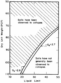
Structures founded on such soils may be seriously damaged if the soils are inundated and collapse. Therefore, if a soil is suspected to be collapse susceptible, then it is of primary importance to estimate the magnitude of potential collapse that may occur if the soil becomes wetted. To do this, a one-dimensional collapse potential test can be performed in an oedometer on undisturbed or recompacted samples according to ASTM D 5333. For this test, a sample is placed in an oedometer at it natural or compacted moisture content and the vertical pressure on the sample is increased in increments to the anticipated final loading in the field. Readings of vertical deformation are taken during the loading sequence. At the anticipated final load level, water is introduced to the sample and the resulting deformation due to collapse is recorded. The percent collapse (%C) is defined as:

where ΔHc is the change in height upon wetting and Ho is the initial height of the specimen. Conceptually, C is a strain. Therefore, for a soil layer with a given thickness, H, the settlement due to collapse, scollapse, if the entire thickness is inundated may be calculated as:

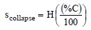
The collapse potential (CP) is calculated as the percent collapse (%C) of a soil specimen subjected to a total load of 4 ksf (200 kPa) as measured by using procedures specified in ASTM D 5333. The CP is an index value used to compare the susceptibility of various soils to collapse. Table 1-12 provides a relative indication of the degree of severity for various values of CP.

1.7.3 Expansion of Soils due to Frost Action

The expansion of soils due to frost action is commonly known as frost heave. Three conditions are required for frost heave to occur. These are (a) freezing surface, (b) source of water, and (c) fine grained soils in which capillary rise can occur. Frost action in soils can have important engineering consequences as follows (after Holtz and Kovacs, 1981):

• The volume of the soil can immediately increase about 10% just due to the volumetric expansion of water upon freezing.
• The formation of ice crystals and lenses in the soil can cause heaving and damage to light surface structures such as small buildings, and highway pavements. Frost action can also displace retaining walls due to increased lateral pressures.

When water in saturated fine-grained soils freezes, it forms lenses of ice oriented roughly parallel to the surface exposed to low temperature (Terzaghi, et al., 1996). Due to the inherent variability in the distribution of pore space, soils affected by frost action do not freeze and expand uniformly. Therefore, just as with swelling and collapsing soils, differential movement occur, and causes structural damage. Upon thawing, the moisture content of the soil increases which leads to reduction in shear strength and a consequent reduction in bearing capacity. Thus, the freeze-thaw cycle results in significant distress to structures and in particular highway pavements.

Only fine-grained soils are susceptible to frost action. However, the critical grain size marking the boundary between soils that are subject to ice-lens formation and those that are not depends on the uniformity of the soil, i.e., the distribution of pore space. The following conditions noted by Terzaghi, et al. (1996) may be used as a general guide for evaluating the frost susceptibility of soils:

• In perfectly uniform soils, i.e., a single particle size soils, ice lenses do not develop unless the grains are smaller than 0.01 mm.
• Uniform soils must contain at least 10% of grains smaller than 0.02 mm.
• In mixed-grain soils, ice lenses form when grains with a size less than 0.02 mm constitute at least 3% of the total aggregate.
• In soils with less than 1% of grains smaller than 0.02 mm, ice lenses are not formed under any conditions which may be encountered in the field.

Common frost susceptible soils include silts (ML, MH), silty sands (SM), and low plasticity clays (CL, CL-ML). One of the most common methods to mitigate the detrimental effects of frost is to place the foundations below the anticipated frost depth. The depth of frost action depends primarily on air temperature below freezing and duration, soil permeability and soil water content. Figure 1-29 can be used for a preliminary estimate of the frost depth. More positive measures to mitigate damage due to frost action include lowering of the ground water table and, depending on the depth of the frost penetration, removal of the frost susceptible soils in the subgrade or foundation. Use of impervious membranes, chemical additives, and even foamed insulation (Styrofoam) under highways, buildings, and railroads have been successfully employed (Holtz and Kovacs, 1981).

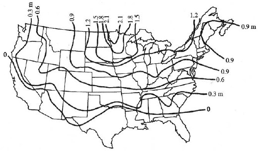
1.8 Compaction Characteristics of Soil

1.8.1 Concept of Compaction

In the construction of highway embankments, earth dams, retaining walls, structural foundations and many other facilities, loose soils must be compacted to increase their densities. Compaction is the process of densifying soil under controlled moisture conditions by application of a given amount and type of energy. Compaction increases the density of the soil, which generally leads to:

• an increase in the strength and stiffness characteristics of the soil,
• a decrease in the amount of undesirable settlement of structures under both static and dynamic loads,
• a reduction in soil permeability, and
• an increase in the stability of slopes and embankments.

Unless compaction is properly controlled, there is a potential that the volume change phenomena described in Section 1.7 (swell, collapse and frost heave) can occur.

The density of compacted soils is measured in terms of the dry unit weight, γd, of the soil. The dry unit weight is a measure of the amount of solid materials present in a unit volume of soil. The greater the amount of solid materials, the stronger and more stable the soil will be. Pertinent parameters for evaluating the results of laboratory and field compaction tests are:

• dry “density” or dry “unit weight.”
• compaction water content.
• type of energy input, e.g., impact, static, vibratory, kneading.
• amount of energy input expressed in ft-lbs/ft³ .

Table 1-13 presents a summary of the characteristics of the most commonly used laboratory compaction tests. Figure 1-30 shows a typical hammer and a mold which is used for performing compaction tests in the laboratory. A comparison of the various values in Table 1-13 reveals that the energy level in the Modified Proctor compaction (MPC) test is 4.5 times that for the Standard Proctor compaction (SPC) test.

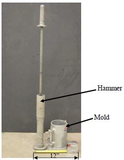
1.8.2 Test Procedures

At least 3 (preferably 5) samples of the same type of soil are prepared at various water contents and compacted according to the requirements listed in Table 1-13. Following compaction, the moist unit weight of the compacted soil (γ_t) in the mold is easily calculated as the weight of the soil (measured) divided by the volume of the mold (constant = 1/30 ft³). The water content (w) is determined as per ASTM D 2216-05 and the dry unit weight is then calculated as:

The dry unit weight (pcf (kN/m3)) for each compacted sample is plotted versus its compaction moisture content (%). The resulting curve is called a compaction curve. Figure 1-31 shows compaction curves for the same soil using Standard Proctor compaction (SPC) test parameters and Modified Proctor compaction (MPC) test parameters as listed in Table 113. The typical compaction curves as presented in Figure 1-31 have the following characteristics:

• Maximum dry density (γ_d-max) is the dry density corresponding to the peak of the compaction curve for a given type and amount of input energy. Note from Figure 131, that the SPC γ_d-max is less than the MPC γ_d-max. Note from Table 1-13 that although the type of energy (impact) is the same for both SPC and MPC, the amount of energy in the MPC test is 4.5 times that of the SPC test.
• Optimum moisture content (w_opt) is the compaction water content at which the soil attains its maximum dry density for a given input energy. Note from Figure 1-31, that the SPC w_opt is greater than the MPC w_opt.

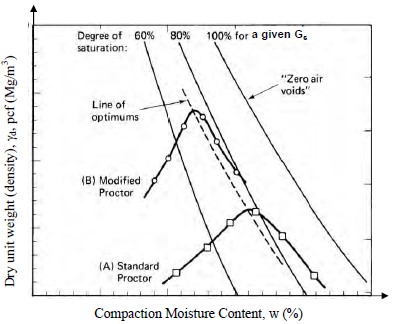
• Zero air voids curve is the curve that corresponds to S=100% regardless of the amount or type of energy input. The importance of the zero-air-voids curve is that it denotes the limits of compaction, i.e., if the moisture content of a fill is too high for a given amount of input energy, the compacted fill may begin to “pump” as its voids become fully saturated with moisture. This can happen even at low moisture contents if the input energy is very large as may be the case with too many passes of a too heavy a piece of compaction equipment. Points on the zero air voids curve are calculated from the basic equation for dry unit weight given by Equation 1-18 by setting S=1 and choosing arbitrary values of compaction moisture content within the range of the compaction curve.

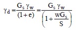
where:

• G_s = specific gravity of solid particles γ_w = unit weight of water
• e = void ratio
• w = water content expressed as a decimal
• S = degree of saturation expressed as a decimal.

Note that the S=100% (zero air voids) curve is calculated for a specific value of G_s, in this case 2.7. Curves corresponding to other degrees of saturation can be calculated in the same way by setting S=80 for the 80% saturation curve, S=60 for the 60% saturation curve and so forth. The saturation curve for a degree of saturation less than 100% is often useful for developing compaction specifications for silty soils since such soils frequently have sharply peaked compaction curves. Therefore, they can begin to “pump” even though the degree of saturation is less then 100%.

• Line of optimums – As its name suggests the “line of optimums” is obtained bypassing a curve through the peaks of the compaction curves that were developed for a certain type of soil compacted at various energy input levels. Testing laboratories frequently develop such curves for various types of soil based on information in their job files. The line of optimums can be used as a guide for developing compaction specifications where no laboratory test data are available.

The above observations are true for all types of soils and apply to all methods of compaction. The most important concept about compaction curves as discussed above is that an increase in the amount of compaction (more energy) results in an increase in the maximum dry density and a corresponding decrease in the optimum moisture content. Therefore, this concept should be recognized when the geotechnical specialist is required to develop specifications for field compaction of soils.

1.8.3 Implication of Laboratory Tests on Field Compaction Specifications

With reference to Figure 1-31 it is obvious that for a given compaction curve the same dry unit weight can be obtained at two different compaction moisture contents, one below optimum and the other above optimum. For fine-grained soils this difference in moisture contents relates to a difference in soil structure that may affect engineering properties such as shear strength and permeability.

It is very important that compaction specifications be given in terms of three parameters: the compaction energy (Standard or Modified Proctor), the desired dry density expressed as a percentage of the maximum dry density, and the compaction moisture content expressed as a range (+ or -) with respect to the optimum moisture content. For example, since the input energy of Modified Proctor is greater than the input energy of Standard Proctor (see Table 113) the Modified Proctor curve plots above the Standard Proctor curve so that 95% of MPC γ_d-max may be greater than 100% of SPC γ_d-max. Likewise, a compaction moisture content of 1 or 2% above optimum for modified Proctor compaction may be below the standard Proctor optimum moisture content. Unfortunately, laboratory compaction curves mainly serve as guidelines for field compaction. This approach is inconsistent because the impact type of energy input in the laboratory is not the same as the type of energy delivered by the equipment commonly used in construction. Figure 1-32 illustrates this point by presenting the types of compactive effort (static, vibratory, kneading) corresponding to the equipment typically used in practice. Note that none of the compaction processes in Figure 1-32 involves impact type of energy that is used to determine the compaction characteristics of the soils in a laboratory SPC or MPC test.

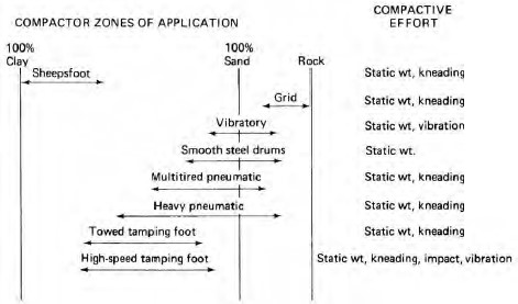
Due to the obvious disconnect between the types of energy in the laboratory and the field, some method is needed to express the laboratory-measured compaction parameters, i.e., maximum dry unit weight (γ_d-max) and optimum moisture content (w_opt), in terms of field compaction. Most commonly, this relationship is achieved by so-called performance based or end-product specifications wherein a certain relative compaction, RC, also known as percent compaction, is specified. The RC is simply the ratio of the desired field dry unit weight, γ_{d field}, to the maximum dry density measured in the laboratory, γ_{d max}, expressed in percent as follows:

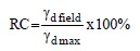
The relative compaction, RC, is not the same as relative density, D_r. Relative density applies only to granular soils with fines less than 12% (ASTM D 2049), while relative compaction is used across a wide variety of soils. Lee and Singh (1971) published the following relationship between RC and D_r based on a statistical evaluation of 47 different granular soils compacted by using Modified Proctor energy (Wright, et al., 2003).

Assuming a linear interpolation, the above relationship can be expressed as follows:

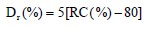
or

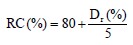
In terms of Standard Proctor, Equations 5-20 and 5-21 are approximately as follows:

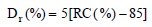
or

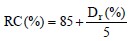
Figure 1-33 presents the above equations in a graphical format. Table 1-14 presents the values of D_r for values of RC values ranging from 85% to 100% for MPC and from 90% to 105% for SPC.

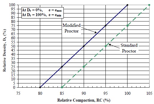
Figure 1-33 and Table 1-14 indicates that for every 1% increase in RC, the increase in D_r is 5% regardless of compaction energy. This is rather significant when it is realized that the shear strength parameter, φ, of granular soils is a direct function of relative density as shown in Figure 1-22 and as illustrated by the following simple computations:

• Based on Figure 1-22, the angle of internal friction for well-graded sands (SW soils)for values of D_r between 50% and 100% varies from 33º to 41º. From Table 1-14,values of D_r between 50% and 100% correspond to RC values of 90 and 100%,respectively for Modified Proctor and 95 and 105%, respectively for Standard Proctor. In other words, for SW soils, for every 1% increase in RC, the angle of internal friction increases by 0.8º.
• Alternatively, the increase in the coefficient of friction, tan φ, would be tan (41º)/ tan(33º) = 1.33 or a 33% increase over a 10% change in RC. In other words, there is a3.3% increase in shear strength for every 1% increase in RC.

Select materials are often specified in the construction of transportation facilities such as embankments, foundations, and pavement sub-bases and bases. The above simple example illustrates the importance of carefully specifying RC for such materials. RC values of 90 to 100% of standard Proctor values are commonly used. Based on Table 1-14, this range of RC corresponds to a D_r between 25% and 75%.

For most transportation applications, the RC value is prescribed in performance based specifications. In this case, it does not matter which equipment or type of compaction energy the contractor chooses to use as long as the end-product meets the specified RC. The prudent contractor would choose the equipment according to the type of soil. Often the contractor chooses to use the equipment he/she owns or is cheapest to lease or rent. Unfortunately, this equipment may not always be the most efficient equipment for the work. Figure 1-32 can be used as a preliminary guide in selecting the type of equipment and mode of compaction energy as a function of soil type. In Figure 1-32 the “100%” above the word clay on the left and the word sand on the right indicates boundaries for the range of soils types in between, e.g. 100% clay means that the soil to be compacted is all fine grained, therefore use of a sheepsfoot roller is recommended. The figure also suggests that a sheepsfoot roller can be used for various soil mixtures consisting of up to approximately 35% fine grained soils and 70 % coarse grained soils.

An example of the influence of the choice of compaction equipment and energy is shown in Figure 1-34. Assume that Curve 1 is obtained from laboratory tests to develop the compaction curve for a borrow material that the contractor has identified for a given project. Further assume that the specification for the project requires that RC = 90%. If M represents the point of maximum dry density, γdmax, then RC=90% would mean that Points P and Y represent the limits of Curve 1 within which the contractor has to operate. In other words, the contractor cannot use compaction moisture contents less than a or c on the compaction moisture content axis.

To properly evaluate the choice of the compaction equipment, the contractor should perform compaction tests at various RC values in the laboratory to develop a line of optimums and a family of curves similar to Curve 2 and 3 shown in Figure 1-34. Once this data is developed, then it can be observed from Figure 1-34, that the most economical water content would be that corresponding to point R along the line of optimums, i.e., the moisture content given by Point b on the X-axis. Point R represents the minimum compactive effort to attain RC=90%. To avoid inadequate compaction and risk failed field quality control tests, a prudent contractor usually aims to achieve somewhat higher dry density. Thus, the contractor often chooses to select a target curve similar to Curve 2 and aim to maintain moisture content in Zone B.

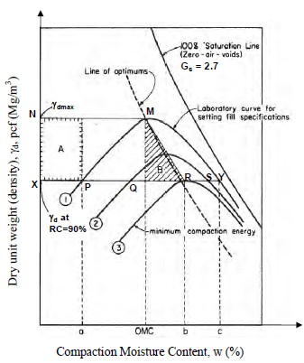
1.8.4 Engineering Characteristics of Compacted Soils

Typical values for the engineering characteristics of compacted soils are given in Table 1-15. The values of the engineering properties refer to soils compacted to maximum dry density by using the standard Proctor test. The data in Table 1-15 are based on more than 1500 soil tests performed by the Bureau of Reclamation in Denver, CO. The large majority of soils were from 17 western states in the U.S. with some foreign soils (USBR, 1960). The background information for the values in Table 1-15 is given in the notes section of the table.

1.8.4.1 Effect of Increase in Moisture Content on Shear Strength of Compacted Soils

The cohesion values, c′ (as-compacted) and c′_sat (after saturation of compacted soil) listed in Table 1-15 are instructive in the context of the apparent cohesion concept discussed in Section 1.5.1.2. In the soil’s compacted state at optimum moisture content (OMC), the capillary stresses and the apparent mechanical forces assume their peak values at that particular compaction energy. Capillary stress, as discussed in Section 1.5.1.2, is due to surface tension in the water between individual soil grains. The magnitude of capillary stress is larger in fine-grained soils than coarse-grained soils as demonstrated by the increasing values of c′ in Table 1-15 as the soil type changes from granular to fine-grained.

The same trend is observed with the c′ _sat values. However, the values of c′ _sat are approximately 10% (for CH soils) to 40% (for SM soils) of the corresponding c′ values. This drastic reduction in cohesive strength is attributable to the effect of capillary stresses being significantly reduced by the increase in moisture content required to reach saturation resulting in much lower apparent cohesive strengths. The reduction may also represent loss of apparent mechanical forces due to reduction in the interlocking of the particles because of the lubricating effect of water.

Based on the above discussions, it is important to ensure that compacted soils are protected against increases in moisture content because the strength of such soils will decrease with associated detrimental effects on the facilities they support.

1.9 Elastic Properties of Soils

The stress-strain behavior of soils and rocks is highly nonlinear or inelastic. Elastic theory provides a convenient first order approximation to stresses and strains induced in soils by external loads. A pair of elastic constants is required when elastic theory is used to solve such problems, e.g., elastic modulus (E) and Poisson’s ratio (ν), or shear modulus (G) and bulk modulus (B), or some other pair of elastic constants. The pair of E and ν is most widely used since both parameters are readily measurable. Consequently, many of the elastic equations in geotechnical engineering are formulated with this pair. Therefore, typical values of E and ν for soils are presented in this section.

The elastic properties of soils may be measured from laboratory stress-strain curves such as those shown in Figure 1-16. The elastic properties, E_s and ν, of a soil may be estimated from empirical relationships presented in Table 1-16 for preliminary design or for final design where the prediction of deformation is not critical to the performance of the structure, i.e., when the structural design can tolerate the potential inaccuracies inherent in the correlations. The definition of E_s is not always consistent for the various correlations and methods of in-situ measurement. FHWA (2002a) provides additional details regarding the definition and determination of E_s. Where evaluation of elastic settlement is critical to the design of the foundation or selection of the foundation type, in-situ methods such as pressuremeter or dilatometer tests should be used for evaluating the modulus of the impacted strata.

The modulus of elasticity for normally consolidated cohesionless soils tends to increase with depth. An alternative method of defining the soil modulus for granular soils is to assume that the modulus, E_s, increases linearly with depth, starting at zero at the ground surface, in accordance with the following equation:

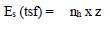
where:

• n_h = rate of increase of soil modulus with depth as defined in Table 5-17 (tsf/ft)
• z = depth in feet below the ground surface (ft)

The formulation provided in Equation 1-24 is used primarily for analysis of lateral response or buckling of deep foundations.

1.10 Common Sense Guidelines for Laboratory Testing of Soils

Sampling and testing of soils is one of the first and most important steps in the design and construction of all types of structures. Omissions or errors introduced here, if undetected, will be carried through the process of design and construction and will often result in costly and possibly unsafe facilities. Table 1-18 lists topics that should be considered for proper handling of samples, preparation of test specimens, and laboratory test procedures. Table 1-18 should in no way be construed as being a complete list of guidelines to avoid possible errors and omissions in handling or testing of soil specimens; there are more. These are just some of the more common ones.

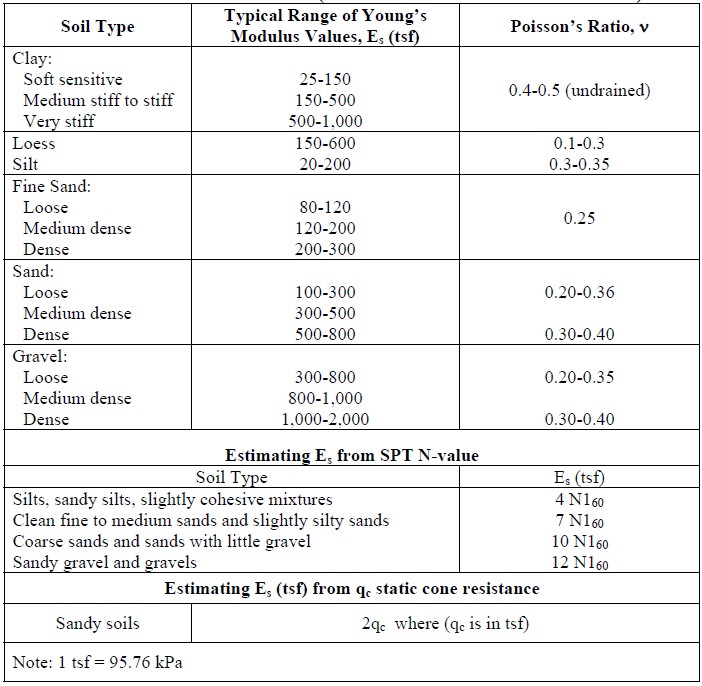
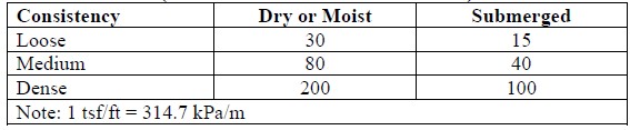
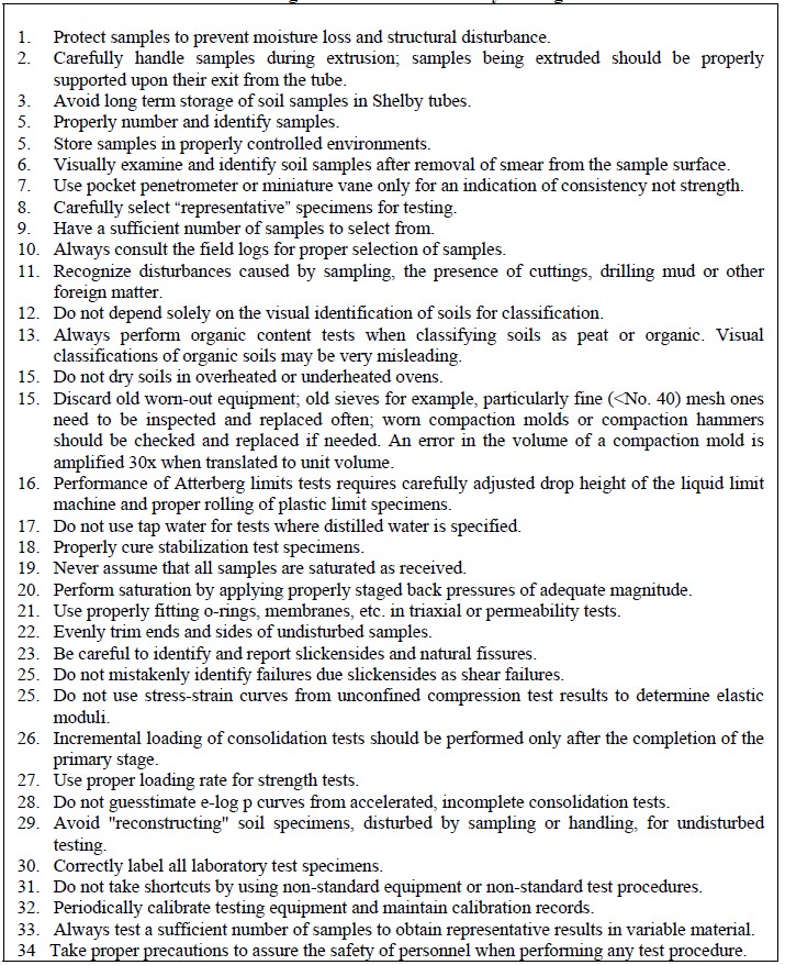
1.11 Laboratory Tests for Rock

1.11.1 Introduction

This section provides information on common laboratory test methods for rock including testing equipment, general procedures related to each test, and parameters measured by the tests. Table 1-19 provides a list of commonly performed laboratory tests for rock associated with typical projects for highway applications. Although other laboratory test methods for rock are available including triaxial strength testing, rock tensile strength testing, and durability testing related to rock soundness, most design procedures for structural foundations and slopes on or in rock are developed based on empirical rules related to RQD, degree of fracturing, and the unconfined compressive strength of the rock. The use of more sophisticated laboratory testing for rock properties is usually limited to the most critical projects. Details on other laboratory testing procedures for rock are provided in FHWA, 1997). Table 1-20 provides summary information on the typical rock index and performance tests.

1.11.2 Point-Load Strength Test

The point load strength test is used to estimate the unconfined compressive strength of rock. Both core samples and fractured rock samples can be tested. The test is conducted by compressing a piece of the rock between two points on cone-shaped platens (see Figure 1-35) until the rock specimen breaks in tension between these two points. Each of the cone points has a 1/5 in (5 mm) radius of curvature and the cone bodies themselves include a 60° apex angle. The equipment is portable, and tests can be carried out quickly and inexpensively in the field. Because the point load test provides an index value for the compressive strength, usual practice is to calibrate the results with a limited number of uniaxial compression tests on prepared core samples. The point load test is also used with other index values to assess the degradation potential of shales.

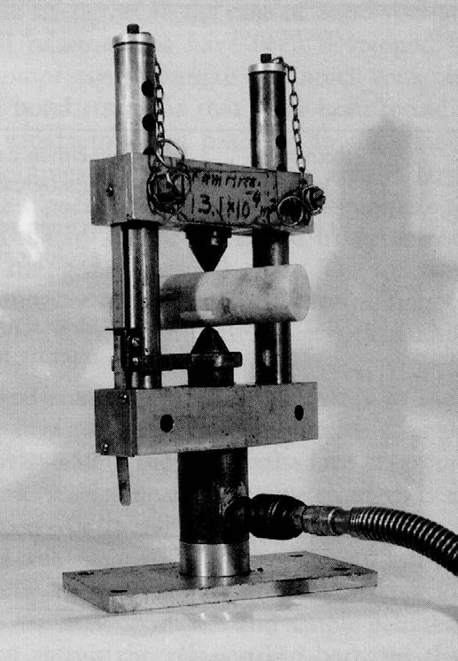
If the distance between the contact points of the platens is D and the breaking load is P, then the point load strength, Is, is calculated as:

where De is the equivalent core diameter given by:

1. De = D² for diametral tests; or
2. De = 4×A for axial, block, or lump tests where A = W×D. The area A is the minimumcross-sectional area of a lump sample for a plane through the platen contact pointswhere W is the specimen width.

The size-corrected point load strength index, I_s(50) of a rock specimen is defined as the value of Is that would have been measured by a diametral test with D = 2 in (50 mm). For tests performed on specimens other than 2 in (50 mm) in diameter, the results can be standardized to the size-corrected point load strength index according to:

The value of the size correction factor, kPLT, is given by:

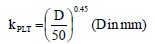
It has been found that, on average, the uniaxial compressive strength, σc, is about 20 to 25 times the point load strength index, with a value of 24 commonly used, i.e.,

However, tests on many different types of rock show that the σ_c / I_s(50) ratio can vary between 15 and 50, especially for anisotropic rocks. Consequently, the most reliable results are obtained if a series of uniaxial calibration tests are carried out. Point load test results are not acceptable if the failure plane lies partially along a pre-existing fracture in the rock, or is not coincident with the line between the platens. For tests in weak rock where the platens indent the rock, the test results should be adjusted by measuring the amount of indentation and correcting the distance D (Wyllie, 1999).

1.11.3 Unconfined Compressive Strength of Intact Rock Core

The unconfined compressive strength of intact rock core can be evaluated by using ASTM D 2938. In this test, rock specimens of regular geometry, generally rock cores, are used. The rock core specimen is cut to length so that the length to diameter ratio is 2.5 to 3.0 and the ends of the specimen are machined flat. ASTM D 2938 provides tolerance requirements related to the flatness of the ends of the specimen, the perpendicularity of the ends of the specimens, and the smoothness of the length of the specimen. The specimen is placed in a loading frame, see Figure 1-36a. Axial load is then continuously applied to the specimen at a uniform rate until peak load and failure are obtained. The unconfined or uniaxial compressive strength of the specimen is calculated by dividing the maximum load carried by the specimen during the test by the initial cross-sectional area of the specimen.

This test is more expensive than the point load strength test, but it is also more accurate with respect to in situ strength. Careful consideration of the design requirements should be made before deciding which test to perform, the unconfined compression test, a performance test, or the simpler point load strength test, an index test.

1.11.4 Elastic Modulus of Intact Rock Core

The test to determine the elastic modulus of intact rock is performed similarly to the unconfined compressive test discussed previously, except that deformation is monitored during application of load. This test is performed when it is necessary to estimate both the elastic modulus and the Poisson’s ratio of the intact rock core. Because of this dual purpose, it is common to measure both axial (or vertical) and lateral (or diametral) strain during compression. It is preferable to use strain gauges glued directly to the rock surface (see Figure 1-36b) as compared to LVDTs mounted on the platens since slight imperfections at the contact between the platens and the rock may lead to movements that are not related to strain in the rock (Wyllie, 1999).

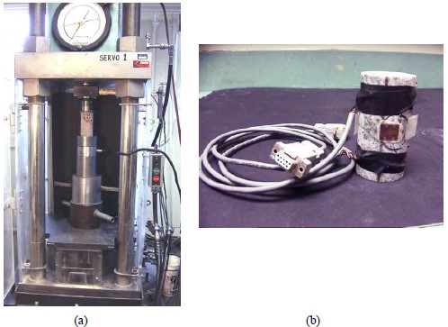
1.11.5 Laboratory Direct Shear Test

The apparatus and procedures for direct shear testing are discussed in ASTM D 5607. The direct shear test is typically used to evaluate the shear strength of a rock discontinuity. Overall, the equipment for the direct shear test on rock is similar to that for soil including a direct shear testing machine, a device for applying normal pressure, and vertical and horizontal displacement monitoring devices. A schematic of the test set up is shown in Figure 5-37. For testing rock specimens, an encapsulating material such as a high strength gypsum cement is poured around the specimen in the upper and lower holding ring. The specimen is sheared as one holding ring is displaced horizontally with respect to the other such that the discontinuity surface is exactly parallel to the direction of the shear load. Load cells are used to monitor the shear force and LVDTs or dial gauges are used to monitor both horizontal and vertical deformation. Multiple LVDTs should be used to monitor vertical deformation and potential rotation of the specimen in the vertical plane.

Typically, the results of a direct shear test on rock are presented on two separate plots: one a plot of shear stress versus shear displacement and the other a plot of normal displacement versus shear displacement. Normal stresses should be adjusted to account for potential decreases in the shear contact area. After the sample is sheared, the sample is reset to its original position, the normal load is increased, and another test is performed. Each test will produce a pair of shear stress and normal stress values for both peak and residual conditions. The friction angle of the discontinuity surface can be evaluated from this data.

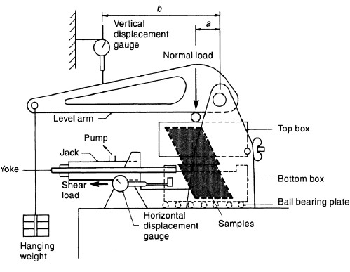
1.12 Elastic Properties of Rocks

Preliminary estimates of the elastic modulus of intact rock can be made from Table 1-21. Note that some of the rock types identified in the table are not present in the U.S. It is extremely important to use the elastic modulus of the rock mass for computation of in-situ displacements of rock under applied loads. Use of the intact modulus will result in unrealistic and unconservative estimates of displacement. Section 1.12.1 presents some guidance for estimating the elastic modulus of a rock mass.

Poisson’s ratio for rock should be determined from tests on intact rock core. Where tests on rock core are not practical, Poisson’s ratio may be estimated from Table 1-22.

1.12.1 Elastic Modulus of Rock Mass

The elastic modulus of a rock mass (E_m) shall be taken as the lesser of the intact modulus of a sample of rock core (E_i) or the modulus computed from one of the following equations:

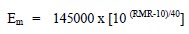
where:

• E_m = Elastic modulus of the rock mass (psi)
• RMR = Rock Mass Rating

Note that in almost all cases, the elastic modulus of the rock mass, E_m, is less than the elastic modulus of the intact rock, E_i.

The elastic modulus of the rock mass can also be determined from the following equation:

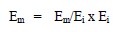
where E_i is the elastic modulus of the intact rock. E_m/E_i is basically a reduction factor to account for discontinuities in the rock mass and can be determined by using the guidance in Table 1-23. In using Table 1-23, it is important that the elastic modulus for the intact rock, E_i, be determined from tests rather than by using the data in Table 1-21. For critical or large structures, determination of rock mass modulus (E_m) by in-situ tests may be warranted. A discussion of suitable in-situ tests can be found in FHWA (2002a).

1.13 Common Sense Guidelines for Laboratory Testing of Rocks

As with soils, omissions or errors introduced during laboratory testing of rock, if undetected, will be carried though the process of design and construction and will often result in costly and possibly unsafe facilities. Table 1-24 lists topics that should be considered and given proper attention so that a reasonable assessment of the rock properties will be assured and an optimization of the geotechnical investigation can be realized in terms of economy, performance, and safety. Guidance in proper handling and storage of rock cores may be found in ASTM D 5079.

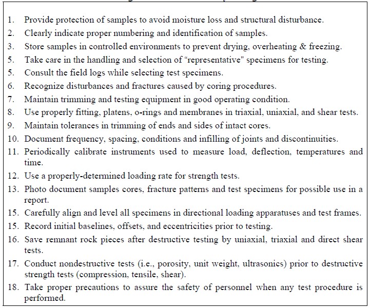
1.14 Practical Aspects for Laboratory Testing

A poor understanding sometimes exists among geologists, structural engineers, and some foundation engineers about the type and amount of laboratory testing required for design of geotechnical features whether they happen to be structural foundations or earthwork. This weakness may render subsequent analyses useless. Organizations that have neither the proper testing facilities nor trained soils laboratory personnel should contract testing to competent AASHTO/ASTM certified private testing firms. This solution can be effective only if the project foundation designer can confidently request the necessary testing and review the results to select design values. A fair estimate of the costs associated with a private testing laboratory may be obtained by assuming the following number of person-days (pd) per test and multiplying by current labor costs:

• visual description of an SPT sample including moisture content (0.05 pd),
• visual description of a tube sample including moisture content and unit weight (0.1pd),
• classification tests (0.7 pd),
• undrained triaxial test (0.9 pd),
• drained triaxial test (2.0 pd),
• consolidation test (2.0 pd).

These values include all work required to present a completed test result to the foundation designer. Alternatively, most private testing laboratories provide a schedule of services and associated costs that can be used to obtain a more accurate estimate of the cost of a proposed laboratory test program.

Blanket consultant contracts “to perform testing necessary for design” usually result in unnecessarily large quantities of testing being performed, much of which does not apply to the project geotechnical issues. For example, if a multi span structure is crossing an area having a soft clay surface deposit underlain by sands, inordinate amounts of time and money should not be spent to determine the strength and consolidation parameters of the soft clay layer at pier and abutment locations in great detail. Generally a pile foundation will be designed by using SPT N-values and the only laboratory testing that may be needed in the soft clay layer may be to estimate drag forces on the piles. Also, non-standard strength testing such as torvanes, penetrometers, etc., which are not covered by ASTM or AASHTO standards, should not be permitted. Such devices should be used only for field index tests to determine consistency.

1.15 Variability of Measured Properties

Table 1-25 presents the values of the coefficient of variation of measured properties that should be taken into consideration as the subsurface model is finalized for engineering design. The data in Table 1-25 can be used by the geotechnical specialist as follows:

• Perform sensitivity (parametric) studies to evaluate the effect of variability in properties with respect to the subsurface profile and the type, magnitude and direction of the anticipated loading and establish the best-case and worst-case scenarios,
• Evaluate the need to perform additional explorations,
• Exercise judgment with respect to the results of engineering analyses and designs and convey the uncertainty to the project team, in particular to the structural engineer, and
• Establish the need for instrumentation to monitor the performance of the facility during and after construction.

The finalization of the subsurface model should be performed by a geotechnical specialist who is experienced in the design and construction aspects of the proposed facility. Active input should be sought from the field inspectors and the laboratory personnel who were actually involved in the collection of the data. At this stage, it is recommended that the geotechnical specialist seek a peer review from one or more qualified and experienced geotechnical specialist(s) with the specific purpose of having them evaluate whether or not the collected data and subsurface model is adequate to permit a cost-effective design of the facility. The experienced geotechnical specialist(s) can also provide information on potential value analysis alternatives (value engineering) for the design of the facility based on the collected data. The importance of such peer reviews cannot be overemphasized. Finally, the owner of the facility should be informed of the findings so that the owner can make decisions such as authorizing more field explorations and/or laboratory tests or modifying the facilities as appropriate based on the results of the geotechnical investigation thus far.